
Figure 1.1 Interrelationships in a fluvial system.
After Thoms (1998) and ideas presented in Schumm (1977) and Knighton (1984).
As of January 2004 au.riversinfo.org is archived under Precision Info
RIVERSINFO AUSTRALIA ARCHIVE
This archive provides non stylised versions of selected reference documents (formerly) resident on au.riversinfo.org.
Melissa Parsons, Martin Thoms, Richard Norris
Cooperative Research Centre for Freshwater Ecology
University of Canberra February 2001

2. Reference Site Selection Procedure
5. Instructions For The Measurement Of Each Variable
This document draws heavily on published stream assessment methods currently in use in Australia and overseas. Thus, we would like to acknowledge the authors of these methods because this document is somewhat a summary of their expertise. These authors are:
River Habitat Audit Procedure
John Anderson
Index of Stream Condition
Tony Ladson, Lindsay White, CRC for Catchment Hydrology and Department of Natural Resources and Environment, Victoria.
River Styles
Gary Brierley, Kirstie Fryirs, Tim Cohen and others at Macquarie University
Habitat Predictive Modelling
Nerida Davies, Martin Thoms, Richard Norris
River Habitat Survey
P. Raven, N. Holmes, F. Dawson, P. Fox, M. Everard, I. Fozzard, K. Rouen and others at the UK Environment Agency and Scottish Environment Protection Agency
AUSRIVAS
All involved with the AUSRIVAS component of the National River Health program at both a State and Federal level. Particular thanks to members of the current AUSRIVAS team at the CRCFE in Canberra for help with the construction of this document: Julie Coysh, Phil Sloane, Sue Nichols, Nerida Davies and Gail Ransom.
USEPA Habitat Assessment
James Plafkin, Mike Barbour, Kimberley Porter, Sharon Gross, Robert Hughes, Jeroen Gerritson, Blaine Snyder, James Stribling
Participants in the Habitat Assessment Workshop also provided ideas for the development of this protocol. These people are:
John Anderson, Rebecca Bartley, Andrew Boulton, Gary Brierley, Nerida Davies, Jenny Davis, Barbara Downes, Fiona Dyer, Wayne Erskine, Judy Faulks, Brian Finlayson, Kirstie Fryirs, Chris Gippell, Bruce Gray, Kathryn Jerie, Tony Ladson, Richard Marchant, Leon Metzeling, Richard Norris, Melissa Parsons, Mike Stewardson, Mark Taylor, Jim Thompson, Martin Thoms, Simon Townsend and John Whittington.
John Foster, Heather McGinness, Vic Hughes, Andrew Pinner and Fiona Dyer of the River and Floodplain Laboratory, University of Canberra, provided advice on several of the variables included in this protocol, and also provided many photographs. Desley Ferguson and Melanie Saxinger provided administrative support.
The physical assessment of stream condition lies within a broad framework of environmental restoration. Most river rehabilitation methods recommend the use of a pre and post-restoration assessment of condition. For example, the 12-Step rehabilitation process of Rutherfurd et al. (2000) includes description of present stream condition and evaluation of the success of the rehabilitation process. Similarly, Kondolf (1995) recommends the collection of baseline data that can be used to evaluate change caused by rehabilitation projects and Hobbs and Norton (1996) stress the importance of identifying the processes leading to degradation or decline, and of developing easily observable measures of the success of restoration interventions. The assessment protocol described in this document addresses these aspects of river rehabilitation by providing a quantitative approach to the physical assessment of river condition.
The Australian River Assessment System (AUSRIVAS) is a nationally standardised approach to biological assessment of stream condition using macroinvertebrates, that was developed under the auspices of the National River Health Program (NRHP). Within the AUSRIVAS component of the NRHP a suite of 'toolbox' projects have been commissioned with the aim of either refining the existing assessment techniques, or developing additional aspects of river health assessment. One of these toolbox projects is the physical assessment module, which involves development of a standardised protocol for the assessment of stream physical condition. Construction of such a protocol requires simultaneous consideration of stream condition from a physical and a biological 'habitat' perspective. While there would seem to be obvious interdependencies between the physical and biological components of streams, merging them is a complex task because of the different paradigms that exist in the disciplines of fluvial geomorphology and stream ecology. However, it is envisaged that the incorporation of a physical assessment module into AUSRIVAS will provide a tool for evaluating and understanding the physical condition of streams that is complementary to measures of stream condition that are made using the biota (Maddock, 1999). This tool can be used to enhance the AUSRIVAS assessments of stream condition, and also to evaluate physical condition within a stream restoration framework.
The AUSRIVAS physical assessment protocol is a method for assessing the physical condition of streams and rivers. The protocol is a 'stand alone' method of physical and geomorphological assessment, however, it also has the capability to complement the biological assessments of stream condition that are made using AUSRIVAS.
This document is essentially a 'field manual' that presents the background information to the method and instructions for the selection of reference sites and collection of physical data. Full implementation of the protocol involves collection of reference site information from both the field and the office, and subsequent development of predictive models. This document describes methods for reference site selection and field and office data collection only. It does not describe methods for the construction of predictive models, because these closely follow the AUSRIVAS procedures described in Simpson and Norris (2000). To make an assessment of physical stream condition using the protocol, a large number of reference sites must be sampled and predictive models generated. Then, the condition of test sites can be determined using these models. This is the same process that was used in the National River Health Program to develop AUSRIVAS.
The protocol follows the Habitat Predictive Modelling approach of Davies et al. (2000) that in turn, is similar to AUSRIVAS in both data collection and analytical procedure (Simpson and Norris, 2000). This approach has advantages over other physical assessment methods in use in Australia because it allows prediction of the stream features expected to occur at a sampling site and generates quantitative assessments of physical condition (ie. observed/expected ratios). However, achievement of robust predictions relies on the inclusion of a wide range of physical and geomorphological factors. Thus, the Habitat Predictive Modelling approach of Davies et al. (2000) will be strengthened with sampling design, data collection and analytical components derived from other physical and geomorphological stream assessment methods presently in use in Australia.
Additionally, it should be noted that this protocol is for use in freshwater rivers and streams only and NOT for use in estuaries or tidal sections of lowland rivers.
This document is divided into seven parts. This section, Part 1, describes the background and derivation of the protocol and also gives an overview of how the protocol works. Part 2 provides information and instruction on the procedure that will be used to select reference sites. These reference sites are then used in the construction of predictive models. Part 3 gives an overview of the requirements for collecting field and office based data and Part 4 contains the data sheets for use in the field. Part 5 is used in conjunction with Parts 3 and 4 and gives detailed technical instructions for the collection or measurement of each field based and office based variable used in the protocol. Part 6 is the reference list and Part 7 contains various appendices to the text.
The protocol has been written with the assumption that the reader is familiar with AUSRIVAS sampling procedures, model development and model outputs. General information on AUSRIVAS can be obtained at http://ausrivas.canberra.edu.au/ and technical information can be found in the papers collected together in Wright et al. (2000).
Development of the physical assessment protocol involved three stages: evaluation of physical stream assessment methods currently in use in Australia, a habitat assessment workshop and derivation of final recommendations for a standardised assessment protocol. Each of these stages will be discussed briefly in the following sections.
The Index of Stream Condition (Ladson and White, 1999; Ladson et al., 1999; White and Ladson, 1999), River Habitat Audit Procedure (Anderson, 1993a; Anderson, 1993b; Anderson, 1993c; Anderson, 1999), River Styles (Brierley et al., 1996; Cohen et al., 1996; Fryirs et al., 1996; Brierley et al., 1999; Brierley and Fryirs, 2000) and Habitat Predictive Modelling (Davies, 1999; Davies et al., 2000) methods were evaluated against a set of criteria that represent the desirable requirements of a standardised physical assessment protocol (Table 1.1).
The Index of Stream Condition, the River Habitat Audit Procedure, River Styles and Habitat Predictive Modelling were designed for slightly different purposes and subsequently, each of these methods differ in their compatibility with the requirements of a standardised physical assessment protocol (Table 1.1). Each method performed equally well against criteria such as 'ability to assess stream condition against a desirable reference state', and 'applicability to all stream types within Australia'. However, only one or two methods performed well against criteria such as 'ability to predict physical stream features that should occur in disturbed rivers and streams' and 'outputs of physical condition that are comparable to AUSRIVAS outputs of biological condition' (Table 1.1). Overall, no one method met all the requirements for a stand-alone stream assessment protocol. However, each method contains important individual components that will be combined into a comprehensive protocol for assessing stream physical condition (see Section 1.2.3).
Twenty-two leading ecologists, geomorphologists and hydrologists attended a workshop titled "Stream Habitat Assessment: Integrating Physical and Biological Approaches", that was held at the University of Canberra on May 2-3, 2000. Broadly, the workshop was designed to provide the rationale and background information upon which to build a standardised physical assessment module. Several critical areas of the development of the physical assessment protocol were identified at the workshop. These were:
In addition, the Habitat Assessment Workshop also examined the types of physical variables that would be useful for inclusion in the protocol.
| Table 1.1 Evaluation of river assessment methods against desired criteria of the physical assessment protocol. The representation of each of the criteria by the methods is designated as yes (Y), no (N) or potentially (P). | ||||
|---|---|---|---|---|
| Criteria required for the physical assessment protocol | Existing physical assessment methods | |||
| River Habitat Audit Procedure | Index of Stream Condition | River Styles | Habitat Predictive Modelling | |
| Ability to predict the physical features that should occur in disturbed rivers and streams | N | N | P1 | Y |
| Ability to assess stream condition relative to a desirable reference state | Y | Y | Y | Y |
| Use of a 'rapid' data collection philosophy | Y | Y | N | Y |
| Use of physical variables that do not require a high level of expertise to measure and interpret | Y | Y | P2 | Y |
| Use of variables that represent the fluvial processes that influence physical stream condition | Y | Y | Y | P3 |
| Outputs that are easily interpreted by a range of users | Y | Y | N | Y |
| Applicability to all stream types within Australia | P4 | P4 | P4 | P4 |
| Incorporation of a scale of focus that matches the scale of biological collection within AUSRIVAS | Y | Y | P5 | Y |
| Collection of physical parameters that are relevant to macroinvertebrates | P | P | P | Y |
| Outputs of physical condition that are comparable to AUSRIVAS outputs of biological condition | N | N | N | Y |
The areas of concern identified at the Habitat Assessment Workshop were considered alongside the evaluation of existing stream assessment methods to make a final set of recommendations for the content and philosophy of the physical assessment protocol. These recommendations were:
These recommendations were then used to formulate the content of the physical assessment protocol (see Section 1.3), including the reference site selection procedure (Part 2) and the methods for field and office based data collection (Part 3).
The philosophy of the physical assessment protocol generally follows the same fundamental principles as rapid biological monitoring programs such as AUSRIVAS. These principles are predictive capability, use of the reference condition concept and use of rapid survey techniques. However, it is also important to incorporate principles of fluvial geomorphology into the protocol because there are fundamental differences between the properties of biological and physical information, and also between the way that information is used within a physically based predictive model. In a biological model, the relationship between physical information and biological information is fundamental whereas in a physical model, the relationship between large scale and small scale physical factors is fundamental (see Section 1.3.2 and Davies et al., 2000). Thus, the incorporation of geomorphological principles that relate small scale and large scale factors underpins the physical model in the same way that the deterministic link between macroinvertebrates and environmental features underpins the biological model. The founding principles of the physical assessment protocol are discussed in the following sections.
RIVPACS is a predictive modelling technique that was developed in the United Kingdom as a tool for the biological assessment of stream condition using macroinvertebrates (Wright, 2000). The predictive modelling approach used in RIVPACS (Wright et al., 1984) forms the basis of AUSRIVAS, the Australian biological assessment scheme that has been used successfully to assess the condition of several thousand sites nationwide (Davies, 2000; Simpson and Norris, 2000). The same predictive technique has also been used for development of the Canadian BEAST predictive models for rivers and lakes (Reynoldson et al., 1997; Reynoldson et al., 2000; Rosenberg et al., 2000) and for the prediction of macroinvertebrate composition using microhabitat features (Evans and Norris, 1997).
Recently, the predictive modelling approach has been applied to the assessment of stream habitat condition (Davies et al., 2000). This study used catchment scale features to successfully predict the occurrence of local scale habitat features and will be used as the basis for the physical assessment protocol. The major advantage to using predictive modelling for assessment of physical stream condition is the ability to predict the local scale habitat features that should be present at a site. Subsequently, it is then possible to compare what is expected to occur at a site, against what was actually observed at a site, with the deviation between these two factors being a quantitative indication of physical stream condition.
There are many interrelated geomorphological factors that operate within a river system. These geomorphological factors sit within a hierarchy of influence (Figure 1.1), where certain factors set the conditions within which others can form (de Boer, 1992; Bergkamp, 1995). Geology and climate are considered ultimate factors because they directly or indirectly control the formation of all other factors in the cascade (Schumm and Lichty, 1965; Lotspeich, 1980; Knighton, 1984; Frissell et al., 1986; Naiman et al, 1992; Montgomery, 1999). Geology and climate act to control to physiography of the catchment, the types of vegetation and soils that are present in a catchment, and the uses to which humans put the land. These factors control sediment and discharge regimes which in turn, sets the morphology and dynamics of the river system (Figure 1.1). Thus, in a fluvial system, physical and geomorphological factors operating at one level of the hierarchy directly influence the formation of factors at successively lower levels.
As a result of this hierarchy of influence within a river system, the deterministic links between different hierarchical levels, or scales, can be harnessed into 'raw material' for a predictive model. For example, Davies et al. (2000) used large-scale catchment characteristics to predict local-scale habitat features in an AUSRIVAS style predictive model and hence, was able to assess habitat condition. Similarly, Jeffers (1998) examined the River Habitat Survey Data (Raven et al., 1998) and was able to predict local-scale habitat features from the map-derived large-scale factors of altitude, slope, distance to source and height of source. The physical protocol will incorporate the hierarchical links within a river system by using large-scale characteristics (or control variables) to predict local-scale habitat features (or response variables, and See Part 3).
In addition to the deterministic links between geomorphological factors at different scales, the hierarchy of geomorphological interrelationships within a river system gives rise to the concept of hierarchical organisation of river systems. Probably the most familiar application of this concept is the stream classification framework of Frissell et al. (1986), which was designed to encompass the relationships between a stream and its catchment at a range of spatial and temporal scales. Five hierarchical levels were named in this scheme: stream systems, segment systems, reach systems, pool-riffle systems and microhabitat systems (Figure 1.2). Each system develops and persists at a characteristic spatial and temporal scale and smaller-scale systems develop within the constraints set by the larger-scale systems of which they are a part (Frissell et al., 1986). The spatial and temporal scales associated with each system subsequently translate into a set of defining physical factors that can be used to identify the hierarchical boundaries of each system within a watershed (Figure 1.2). For example, at the top of the hierarchy, stream systems within a watershed persist at large spatial scales and long time-scales (Figure 1.2) and are defined partly by ultimate factors such as geology and climate. This pattern of characteristic scales of persistence and physical factors continues through the hierarchy of segment, reach and pool/riffle systems until at the bottom of the hierarchy, microhabitats persist at small temporal and spatial scales and are defined by dependent factors such as substrate, water velocity and water depth (Figure 1.2). Thus, the division of a catchment into component hierarchical systems provides a practical representation of the complex interrelationships that exist between physical and geomorphological factors across different spatial and temporal scales.

| Figure 1.2 Hierarchical organisation of a stream system, and its habitat sub-systems. The approximate linear spatial scale (metres) and time scale of persistence (years) for a second or third-order mountain stream is also indicated for each system. After Frissell et al. (1986). |
In the physical assessment protocol, data are collected at two spatial scales: a large catchment or segment-scale and a small sampling site scale. As mentioned above, large-scale factors are then used to predict the occurrence of small-scale factors. While these scales of measurement represent the deterministic links between geomorphological factors at different scales, they also correspond to the stream system or stream segment, and reach or pool/riffle scales of Frissell et al. (1986; and see Figure 1.2). Thus, the scales of measurement used in the protocol target differences between these specific hierarchical levels. The microhabitat is not considered as an explicit scale of measurement, because the protocol does not aim to predict physical factors at this level of detail. Additionally, the stratification of reference sites by regions and functional zones (see Part 2) is a function of the hierarchical organisation of river systems. Geomorphological processes related to the formation of regions and functional zones operate over large spatial scales and long time-scales and thus, sit at the top of the hierarchy (Figure 1.2). As a result, reference site stratification is targeted at the catchment and segment scales, because it is desirable to identify the broad (rather than fine) differences in river types that occur at these relatively large scales. Stratification of reference sites across a framework derived from geomorphological process will also ensure coverage of a range of deterministic linkages between large and small scale variables, that may change across regions and functional zones (Schumm, 1977).
The physical assessment protocol uses the reference condition concept. The reference condition concept underpins many biological assessment programs including the United Kingdom's RIVPACS, Australia's AUSRIVAS and Canada's BEAST predictive models (Reynoldson et al., 2000). The reference condition concept circumvents reliance on single control sites, and instead, aims to derive large sets of minimally disturbed reference sites that are formed into groups with similar biological and physical features (Reynoldson and Wright, 2000). Hence, the reference condition is defined as 'the condition that is representative of a group of minimally disturbed sites organised by selected physical, chemical and biological characteristics' (Reynoldson et al., 1997). Assessment of condition is subsequently achieved by comparing a test site against a group of multiple reference sites that would be expected to have similar features in the absence of degradation. Comparison of a test site against a reference condition derived from multiple sites improves confidence that observed degradation results from anthropogenic factors, rather than from inherent natural variation.
The reference condition concept was derived from work in the field of biological assessment of stream condition (Reynoldson and Wright, 2000), and has been applied successfully to the development of models that assess habitat condition (Davies et al., 2000). However, in applying the reference condition concept to physical assessment of stream condition there are two specific aspects that need to be considered: coverage of a range of different river types and definition of 'minimally disturbed' conditions. Reynoldson and Wright (2000) warn that the population of reference sites must represent the full range of conditions that are expected to occur at all other sites to be assessed. The physical assessment protocol addresses this aspect by stratifying reference sites on the basis of climatic and geological regions, and on the basis of geomorphological river types within regions (see Part 2). Selection of reference sites that represent 'minimally disturbed' conditions is also central to the reference condition concept, and requires consideration of the factors that may be acting to influence stream condition (Hughes et al., 1986; Hughes, 1995; Reynoldson and Wright, 2000). The physical assessment protocol addresses this by examining the large scale and local scale activities that may potentially be impacting the river system (see Part 2).
In the last three decades biological monitoring has moved away from the use of intensive quantitative surveys, toward the use of rapid, semi-quantitative stream assessment methods (Resh and Jackson, 1993). There are two main advantages of rapid survey techniques. Firstly, the effort and cost required to assess environmental condition is reduced relative to that needed in quantitative approaches, by using simplified sampling and sample processing techniques. Secondly, the results of these surveys can be summarised into a form that is easily understood by a range of non-specialists (Resh and Jackson, 1993; Resh et al., 1995). However, in achieving these advantages, the design of rapid methods must maintain an ability to detect a continuum of impaired and unimpaired conditions. Examples of rapid biological monitoring techniques that have been used successfully to examine stream condition include the United Kingdom's RIVPACS (Wright et al., 1984; Wright 2000), the United States' Rapid Bioassessment Protocols (Plafkin et al., 1989; Barbour et al., 1999) and Australia's AUSRIVAS predictive models (Marchat et al., 1999; Smith et al., 1999; Turak et al., 1999; Davies, 2000; Simpson and Norris, 2000).
In recent years, rapid assessment principles have been applied to physical stream assessment methods. Examples include Australia's River Habitat Audit Procedure (Anderson 1993a, 1993b, 1993c) and Index of Stream Condition (Ladson and White, 1999), the United Kingdom's River Habitat Survey (Raven et al., 1998) and the United States' HABSCORE habitat assessment, that is used to support the Rapid Bioassessment Protocols (Plafkin et al., 1989; Barbour et al., 1999). These assessment methods incorporate a range of physical characteristics, representing major geomorphological and habitat-template components. Variables included in these methods are measured using simplified techniques such as visual assessment and overall estimation, rather than the more time-consuming quantitative techniques such as surveying, replicated sedimentological particle size analysis, historical interpretation and transect vegetation surveys. The methods described above have demonstrated that it is possible to achieve a robust assessment of physical stream condition using data collected with rapid survey techniques, and as such, the physical assessment protocol will also use rapid techniques.
River systems can be viewed at distinctive hierarchical levels that represent a cascade of geomorphological interrelationships (see Section 1.3.1.2). The characteristic geomorphological processes that operate at each hierarchical level within a river system create the physical structure of a river (Frissell et al., 1986; Harper and Everard, 1998; Brierley et al., 1999) and in turn, the physical structure of a river provides a habitat matrix within which biophysical processes occur (Swanson, 1979; Brierley et al., 1999; Montgomery, 1999). Biologically, it has been proposed that habitat provides the templet on which evolution acts to forge characteristic life history strategies (Southwood, 1977; Southwood, 1988; Hildrew and Giller, 1994; Townsend and Hildrew, 1994). Accordingly, the environmental properties of any given habitat within a stream system will determine the types of macroinvertebrate communities found there. Therefore, stream habitat forms as a result of characteristic geomorphological processes and so conveniently sits between the physical forces which structure river systems and the biological communities that inhabit them (Harper and Everard, 1998).
There is much evidence to suggest that macroinvertebrates are strongly and deterministically linked to the availability of suitable habitat features. These features include substrate, discharge, hydraulics, riparian vegetation and water chemistry (Giller and Malmqvist, 1998). The physical assessment protocol is designed to complement biological assessments made using AUSRIVAS and thus, it will include factors that are important components of macroinvertebrate habitat. However, most of these environmental factors do not occur randomly within a river system, but rather, exist as a result of a suite of geomorphological processes that operate across a continuum of scales (Figure 1.1). The physical assessment protocol is also designed as a stand-alone method of physical stream assessment and as such, it will include geomorphological aspects of channel character. These channel characteristics may not appear to be directly related to macroinvertebrates, but are important structural and functional components of a river system.
As an overall method of stream assessment, the physical protocol works in a similar manner to AUSRIVAS (Figure 1.3). Physical, chemical and habitat information is collected from reference sites and used to construct predictive models, which are in turn, used to assess the condition of test sites. The physical assessment protocol comprises the following major components:
Reference site selection
Reference sites representing 'least impaired' conditions are selected, and stratified to cover a range of climatic regions and geomorphological river types (see Part 2).
Data collection
Each reference site is visited once and physical, chemical and habitat variables are measured using standardised methods (see Parts 3, 4 and 5). In the office, a suite of predictor variables is measured using standardised methods (see Parts 3 and 5).
Model construction
Predictive models are constructed using the same processes and analyses used in AUSRIVAS (Figure 1.3). However, in the physical assessment protocol, large-scale catchment characteristics are used to predict local scale features (Davies et al., 2000). Thus, the outputs of a physical predictive model are based on the occurrence of local scale features, rather than the occurrence of macroinvertebrate taxa (Figure 1.3).
Assessment of test sites
Assessment of stream condition involves the collection of local scale and large-scale physical, chemical and habitat information from test sites (Figure 1.3). This information is then entered into the predictive models and an observed:expected ratio is derived by comparing the features expected to occur at a site against the features that were actually observed at a site. The deviation between the two is an indication of physical stream condition.
As mentioned in Section 1.1.2, this document contains information on the selection of reference sites, and on the collection of field and office data. It does not provide technical information on the analytical procedures used to construct predictive models from reference site data, because these are documented in Simpson and Norris (2000).
There are several similarities and differences between the AUSRIVAS sampling protocol and the physical assessment protocol. In addition to the elements described in Section 1.3.1, similarities between the two protocols include measurement of similar types of habitat variables (see Part 5), use of some of the same reference sites (see Part 2), use of the same analytical techniques to build predictive models and production of the same model outputs (Figure 1.3). The experiences gained during the seven years of the National River Health Program will be invaluable throughout all stages of the physical assessment protocol.
![Figure 1.3a Overview of the analytical and assessment process used in the physical assessment protocol (left - top) and AUSRIVAS (right - below). [Note: In the original document the top figure (now 1.3a) was left and the bottom (now 1.3b) was right]](../attachments/library/2002/ausrivas_protocol/phys_assess_prot/images/fig1pt3a.gif)
![Figure 1.3b Overview of the analytical and assessment process used in the physical assessment protocol (left - top) and AUSRIVAS (right - below). [Note: In the original document the top figure (now 1.3a) was left and the bottom (now 1.3b) was right]](../attachments/library/2002/ausrivas_protocol/phys_assess_prot/images/fig1pt3b.gif)
|
Figure 1.3 Overview of the analytical and assessment process used in the physical assessment protocol (left - top) and AUSRIVAS (right - below). [Note: In the original document the top figure (now 1.3a) was left and the bottom (now 1.3b) was right] |
Although the outputs of the physical assessment protocol are complementary to the biological assessments made using AUSRIVAS, the protocol is designed to be a stand-alone stream assessment method. Thus, there are several unique preparation, sampling, processing and analytical aspects of the physical assessment protocol that should be noted. The physical assessment protocol differs from AUSRIVAS in the following ways:
The reference site selection procedure for the physical assessment module considers humans to be part of the landscape (Norris and Thoms, 1999) and thus, is based on the concept of 'least disturbed' condition. Collection of reference site information is central to the construction of a predictive model and in turn, this information is used as the baseline against which the condition of test sites is assessed (see Part 1). A reference site selection procedure that uses the concept of least disturbed condition essentially allows for the careful inclusion of sites that have inevitably been affected by humans, but which are considered to be the best available representatives within a certain area or of a specific river type.
The reference site selection procedure described here is similar to that used in the AUSRIVAS program (see Davies, 1994). However, slight modifications have been added to allow for the stratification of reference sites across a range of geomorphological river types. This stratification step ensures that sites from different 'functional zones' are included in the reference site database. Given that local scale habitat features will differ among functional zones (Schumm, 1977), the stratification of reference sites across these zones will ensure representation of the characteristic habitat features that are associated with each zone type. In turn, inclusion of reference sites from different functional zones will strengthen the robustness of predictive models for assessing a range of test sites and human impacts (Reynoldson and Wright, 2000). The existing AUSRIVAS reference sites will be overlain across the zone types and used wherever possible, although additional reference sites may be required in zone types that are currently under-represented.
In addition, the reference site selection procedure has been designed to accommodate several levels of heterogeneity, as a 'safety-net' for the robust construction of predictive models. The site selection procedure will incorporate a regional stratification element as well as a functional zone stratification element, because it is not known in advance whether groups of reference sites will classify on the basis of State or Territory wide regional patterns or on zone type patterns. Thus, regardless of whether reference sites are grouped on the basis of regional or zone type patterns, enough sites will exist in each group to allow the construction of robust predictive models.
The reference site selection procedure assumes that like AUSRIVAS, sampling will be conducted by State or Territory agencies and that ultimately, the predictive models will be set up on a State or Territory basis. Thus, the steps described below should be applied in each State or Territory. The following sections also assume a general familiarity with the concept of 'least impaired condition', as used in the National River Health Program and the development of AUSRIVAS predictive models. The reference site selection procedure consists of six steps:
Each of these steps will be explained in detail in the following sections.
The division of each State or Territory into broad regions allows the stratification of sampling sites across areas with different climatic and geological characteristics.
Within each State or Territory, identify broad climatic regions which have markedly different rainfall and temperature regimes. These broad climatic regions may also have characteristic vegetation patterns. Then, identify broad geological regions. Maps of geological regions can be found on the Australian Geological Survey Organisation's website at http://www.agso.gov.au.
Using primarily the information on broad climatic patterns, and secondarily on geological patterns, delineate a final set of regions that characterise State or Territory wide differences in both factors. The scale of resolution for the final regions should be kept large and broad. For example, a State may contain four major climatic regions, two of which encompass two major geological regions (Figure 2.1). Thus, the State should be divided into six broad climatic and geological regions. The broad climatic and geological regions should be marked onto topographic maps.

River characterisation requires the ordering of sets of observations or characteristics into meaningful groups based on their similarities or differences (Naiman et al., 1992; Wadeson and Rowntree, 1994). Implicit in this exercise is the assumption that relatively distinct boundaries exist and that these may be identified by a discrete set of variables. Although river systems are continuously evolving and often display complexity, the grouping of a set of elements with a definable structure can aid in examining the physical structure of river systems. It may also assist in understanding why rivers have certain biological characteristics.
Geomorphological analyses of river systems often reveal a continuum of functions that change in an upstream-downstream direction. For example, headwater regions often provide a net supply of water and sediment to the river network, while through deposition, lowland alluvial river channels store sediment in vast floodplains. Changes in the flow and sediment regime throughout a catchment will be manifested by changes in river morphology and behaviour. Schumm (1988) suggests that there are three broad functional zones within a catchment:
The geomorphological processes conveyed through these functional river zones will be incorporated into the reference site selection procedure and together with the climatic and geological regions, will form the basis for stratification of sampling sites across the landscape.

For the purposes of the physical assessment protocol, functional zones are defined as lengths of river that have similar water and sediment discharge regimes. Four zone types are recommended in the reference site selection procedure: upper zone A (low energy unconfined), upper zone B (high energy confined), transition zone and lower zone. Water and sediment discharge regimes manifest distinctive geomorphological characteristics in each of these zone types and thus, rivers can be divided into zones using three key indicators of channel character: channel slope, valley character and river channel or planform pattern. This section describes the four functional zone types, and the method used to divide rivers into these zones.
Reference sites will be stratified across four functional zone types. These zone types represent a broad continuum of geomorphological processes occurring within a catchment and thus, will be applicable and valid in the majority of river systems found in Australia. Each zone type will be described in more detail in the following pages.
Upper zone A (low energy unconfined)
Upper zone A is characterised by long pools that are separated by short channel constrictions (ie. chain of ponds morphology). The pools form upstream of the channel constrictions, and are the dominant morphological feature in this zone type (Figure 2.3). Channel constrictions are generally associated with major bedrock bars that extend across the channel, or substantial localised gravel deposits that act as riffle areas. Local riverbed slopes increase significantly at these constrictions, representing small areas of relatively high energy that contrast with the relatively low bed slopes and energies of the pool environment. Overall, bed slope in upper zone A is in the order of 0.0001, with a corresponding stream power in the order of 1.5 W/m2. Stream power (w) is related to the rate at which 'work' (sediment movement) is done or at which energy is expended in a stream or river.
The planform channel configuration of upper zone A is controlled by the valley morphology. Generally, the river channel has a small flanking floodplain (up to 30m) because of the narrow valley floor configuration. Hence, valley conditions limit floodplain development. Bankfull channel dimensions can be up to 30m in width, 3-4 metres in depth/height and may have a width to depth ratio of up to 10. Bankfull channel capacities do not generally exceed 30 m3 s-1.
The nature of channel sediment or substratum in upper zone A consists of fine silt/clay material overlying a bedrock/cobble base in the pools. However, gravel/cobble or bedrock substrates dominate the short constricted riffle areas. Bankfull flows have the competence to entrain the finer bed substratum, however, discharges in excess of 50 m3 s-1 are required to initiate motion of the coarser material. Thus, the riverbed in this zone type is relatively stable because discharges large enough to move coarse materials rarely occur.

Upper zone B (high energy confined)
Upper zone B is a high energy zone dominated by bed slopes greater than 0.002 and often by steep bed slopes greater than 0.010. Bankfull stream power is generally in excess of 250 W/m2 and can exceed 400 W/m2 in steeper sections. Bedrock chutes, large boulder/cobble/gravel accumulations and scour pools dominate in the channel. Bed sediments are relatively immobile because the streambed tends to be armoured (ie. the coarse surface layer sediments shield the finer sediments beneath it). However, cobble and gravel accumulations are highly mobile during flood flows. The lack of any major sedimentary deposits, together with the high energy environment, suggests that upper zone B is an important source of sediment for the downstream river system (Figure 2.4).
Planform channel pattern in upper zone B is confined and controlled by valley morphology, and the river channel generally exhibits an irregularly meandering pattern that is superimposed on a larger valley pattern. Hence, channels in this zone have limited floodplain development. In highly confined sections, the floodplain will be absent and sediments will be added directly to the channel from adjacent valley side slopes. However, in less confined sections, small floodplain formations may be present and are characterised by a series of floodplains of different ages, inset into higher level terraces.

Figure 2.4 Typical example of an upper high energy confined zone.
Transition zone
The transition zone is characterised by mobile bed sediments, large sediment storage areas within the channel and an active channel (Figure 2.5). The presence of well developed inset floodplain features such as benches, point bars, cutoffs and levees signify the relatively active and unrestricted nature of this river-floodplain environment. Valley floor widths of up to 10km enable floodplain development and stream migration.
In the transition zone, the river channel is freely meandering with an irregular planform pattern. Sinuosity is generally between 1.7 and 1.95, and stream power generally ranges from 8 to 20 W/m2. Meander wavelengths are generally less than 2km.
The morphology of the channel environment is extremely variable with bars (point and lateral), benches (at various levels) and riffle/pool sequences present alone or in combination. These in-channel storage features reflect high rates of sediment transport. Riverbed sediments typically have a bimodal distribution (median grain size of 64 to 100mm) and the bed is usually highly mobile.

Figure 2.5 Typical example of a transition zone.
Lower zone
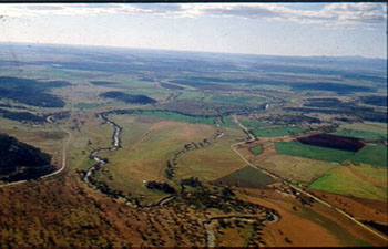
A distinguishing feature of the lower zone is the significant increase in the width of the valley floor (>15km) and associated floodplain surface (Figure 2.6). There are strong and active links between the river and the floodplain, and the lower zone may contain well developed features such as distributary or flood channels (channels that carry water onto the floodplain), former or paleo channels, avulsions, cut-offs or anabranches (channels that dissect the floodplain and rejoin the main channel). The channel displays a typically unrestricted meandering style, with a relatively high sinuosity of about 1.8 to greater than 2.3. Meander wavelengths are approximately 200-700m.
The appreciable fining of bed sediment is a clear distinguishing feature between the transition zone and the lower zone. Bed sediments in the lower zone are typically composed of fine materials such as sand, silt and clay. The bank sediments are also composed of fine materials. As a result, stream banks are often steep in the lower zone and may be naturally susceptible to erosion. The bankfull channel has widths that range between about 30-100m and bankfull depths that range between 3 and 15 metres.


Functional zone types are identified by drawing up long profiles of slope, valley width and planform channel pattern (Figure 2.7). A long profile is a plot of the character of interest against downstream river distance. Long profiles are constructed for EACH river within EACH region, using topographic maps.
The completed long profiles for each river are examined simultaneously to identify the presence of one or more functional zone types (Figure 2.8), according to the characteristics described in Section 2.4.2.1. Supplementary information such as aerial photographs, satellite images, sediment data or local knowledge can also be used to confirm the interpretations of functional zone types from the long profiles. Once identified from the long profiles, the zone types that occur along each river are marked onto topographic maps.

There can be a high level of variability and complexity in the arrangement of functional zone types. The four zone types are broadly sequential along the river continuum, however, the same zone type may be identified more than once in the same river (Figure 2.8). Additionally, it is common for rivers to contain only one or two functional zone types. It is recommended that the division of rivers into functional zone types should proceed according to the above instructions, but in consultation with a geomorphologist.
Figure 2.7 (see next table below) Construction of long profiles for slope, valley width and planform channel pattern. Assessments of each variable are made using topographic maps. Measurements should be taken at regular intervals along the river, according to size and variability. For example, in a 60km long river, measurements should be made every 5km but in a 250km long river, measurements should be made every 10km.
| Long profile | Method | Example profile |
|---|---|---|
| SLOPE | Plot altitude against distance downstream. Altitude (m) and distance from source (km) can be measured off topographic maps. | 
|
| VALLEY CHARACTER | Plot valley width against distance downstream. Valley width is the distance (m) between the first topographic contours, on either side of the channel. Valley width should be measured off the lowest map scale possible. |  |
| PLANFORM CHANNEL PATTERN | Determine the channel patterns that occur along the length of each river, according to the following categories:  |  |
Figure 2.8 (see next below) Interpretation of functional zone types from long profiles. For the zone types, UZA = Upper Zone A, UZB = Upper Zone B, TZ = transition zone and LZ = lower zone. More information on zone types is provided in Section 2.4.2.1.
 |
Breaks in slope, valley width and planform channel pattern are marked on the long profiles. Then, these breaks are assigned to functional zone types, according to the descriptions given in Section 2.4.2.1 and any supplementary information that is available (see Section 2.4.2.3). |
 | The final sequence of functional zone types for this example is UZA � UZB � UZA � TZ � LZ. |
 | The start and endpoints of these functional zones should then be marked on topographic maps. |
Identification of areas that are potentially impacted by large scale and local scale activities allows the elimination of these areas as potential sources of reference sites.
Disturbances that may potentially be impacting the river system are examined at a large catchment scale and at a local scale (see Sections 2.5.2.1 and 2.5.2.2). Sources for obtaining this information on potential disturbances include local managers, experience of agency staff, aerial photographs, hydrology records, GIS maps, and previous data collected for programs such as AUSRIVAS, individual State or Territory projects or the National Land and Water Audit.
Large scale activities are those which have the potential to effect whole catchments within a river system (Table 2.1).
| Table 2.1 Large scale activities to be considered when identifying least impaired areas within river systems. | |
|---|---|
| Activity | Factors to consider |
| Landuse | Percent cover of native vegetation, percent cover of agricultural or grazing land, time since land clearance, degree of impact of land clearance on the downstream river system, percent cover of urban areas, degree of impact of urban areas on the downstream river system, presence of active (<5 years) logging areas, degree of catchment erosion, degree of sedimentation |
| Hydrological regime | Presence of major impoundments, downstream effects of major impoundments, degree of change to flooding regime including magnitude and timing, degree of change to flow seasonality, water extraction activities, reductions or increases in velocity, reductions or increases in discharge sizeIt will be difficult to avoid regulated segments of river in some areas, particularly in lower zones. Where it is impossible to avoid regulation in identifying reference conditions, the overall magnitude of impoundment effects should be considered. |
| Current and historical mining activity | Degree of impact of current mining activities on the downstream river system, degree of impact of historical mining activities on river system character |
Local scale activities are those that may cause localised disturbance to rivers (Table 2.2).
| Table 2.2 Local scale activities to be considered when identifying least impaired areas within river systems. | |
|---|---|
| Activity | Factors to consider |
| Riparian zone characteristics | Presence or absence of riparian vegetation, type of riparian vegetation (native or exotic), influence of exotic vegetation on channel character |
| Channel modification | Channel realignment (straightening or widening etc.), historical incision (ie. severe erosion) of channel, historical infilling (ie. sediment build up) of channel, presence of bridges, fords and culverts and the effects of these on channel character, presence of minor weirs and the effects of these on channel character |
| Desnagging and instream vegetation removal | Historical or recent desnagging, removal of other instream vegetation such as macrophytes |
| Floodplain condition | Connectivity between the river and the floodplain, floodplain erosion, floodplain landuse |
| Human access | Density of public access tracks and roads, location of recreational areas such as camp grounds and picnic areas, presence of road crossings |
| Stock access | Extent of stock access to the channel, impact of stock access on bank condition, impact of stock access on bed condition |
| Bank condition | Extent of non-natural bank erosion, presence or absence of riparian vegetation |
| Point source impacts | Presence of discharge pipes, mining, stormwater discharges, construction sites etc. |
This information on large and local scale activities will be used in Step 5 to determine areas of least impaired condition that are potential sources of reference sites. When using this information it is important to consider the different effects of large scale and local scale impacts. For example, significant forestry activities may occur across a wide area, however, a riparian buffer may exist to protect the stream on a local scale. Conversely, stock may have access to localised patches of river within an otherwise least impaired area and thus, reference sites should not be placed in these localised patches.
Sites assessed by AUSRIVAS as being in good biological condition can be used to indicate areas of river in least impaired condition. It can also be assumed that sites with a healthy biota will have a healthy supporting habitat.
Plot the location of AUSRIVAS reference sites (ie. those sites used to construct the predictive models) and any Band A test site (ie. those sites assessed in the First National Assessment of River Health). Mark these sites onto topographic maps.
The identification of 'least impaired' areas within each region and zone will highlight river sections where reference sites can be placed.
Least impaired areas are identified using the information collected in Steps 3 and 4. In each region and zone, mark onto topographic maps the sections of river that are least impaired. These areas are the sections of river where reference sites can be placed.
It is important to include least impaired areas from all the zone types present within a region. However, it is recognised that in comparison to the upper zones, the transitional and lower zone types will contain lower numbers of least impaired areas because it is usually these latter zone types that are most subject to impact. Thus, stringency of the criteria for determining least impaired areas may change among zone types. Relaxation of least impaired status in the transitional and lower zones should be done using supplementary information from previous biological, chemical or physical surveys, or using best professional judgement.
Stratification of reference sites equally across regions and zones within regions will ensure coverage of a range of geomorphological river types. In turn, this coverage will improve the analytical robustness of the physical predictive models (see Section 2.1).
The recommended total number of reference sites to be sampled in each State or Territory is given in Section 2.9. Regardless of the total number of reference sites used, sampling effort should be divided equally among regions and then among functional zones, according to the relative proportion of each zone type in each region. An example stratification of sampling effort across regions and zones is given in Table 2.3.
The final selection of reference sites is achieved by allocating the desired number of sites across zone types located within the least impaired areas identified in Step 5. Existing AUSRIVAS reference sites should be used where possible, however, additional sites may be required in particular zone types that are not adequately represented in the AUSRIVAS database. Reference sites should also be spread across a range of different rivers within the region.
The number of reference sites required to construct the physical predictive models is roughly the same as that used to construct the AUSRIVAS predictive models. The larger States (NSW, QLD, WA, VIC) should sample 230-250 reference sites (minimum 230) and the smaller States and Territories (ACT, SA, TAS, NT) should sample 180-200 reference sites (minimum 180). These figures represent the number of sites required to build the final predictive models. However, it may be necessary to sample additional reference sites to account for situations where sites are excluded post-hoc because of unexpected impairment.
As there are no strongly overriding temporal or seasonal aspects to the measurement of most physical and habitat features, each reference site only needs to be sampled once. Predictive models can be constructed after a single visit to each sampling site, and the subsequent collection of additional office based information (see Part 3).
| Table 2.3 Example stratification of sampling sites across zones and regions, for a hypothetical State or Territory containing four regions and a total of 200 reference sites. For the zone types, UZA = upper zone A, UZB = upper zone B, TZ = transition zone and LZ = lower zone. | ||
|---|---|---|
| Region 1 (50 Sites) | ||
| Zone type | % zone type in region | Number of sites in each zone |
| UZA | 20 | 10 |
| UZB | 40 | 20 |
| TZ | 30 | 15 |
| LZ | 10 | 5 |
| Region 2 (50 Sites) | ||
| Zone type | % zone type in region | Number of sites in each zone |
| UZA | 10 | 5 |
| UZB | 10 | 5 |
| TZ | 70 | 35 |
| LZ | 10 | 5 |
| Region 3 (50 Sites) | ||
| Zone type | % zone type in region | Number of sites in each zone |
| UZA | 10 | 5 |
| UZB | 0 | 0 |
| TZ | 30 | 15 |
| LZ | 60 | 30 |
| Region 4 (50 Sites) | ||
| Zone type | % zone type in region | Number of sites in each zone |
| UZA | 0 | 0 |
| UZB | 70 | 35 |
| TZ | 25 | 12 |
| LZ | 5 | 3 |
| Total Sites | 200 | |
Once the predictive models are constructed using the reference site information, it will be necessary to 'validate' assessments of physical stream condition using information collected from a small set of test sites. A test site is defined as any site at which condition is assessed using the predictive models. The larger States (NSW, QLD, WA, VIC) should sample 20-30 test sites (minimum 20) and the smaller States and Territories (ACT, SA, TAS, NT) should sample 15-20 test sites (minimum 15). Test sites should initially be stratified across the different regions and zones. Within these areas, test sites should then be located to represent a range of disturbances that may potentially influence physical stream condition.
The sampling design for the physical assessment protocol consists of two aspects. First, reference sites are stratified across the landscape according to broad climatic regions and geomorphological zones (see Part 2). Then, physical, chemical and habitat information is collected locally from each reference site, and in future, each test site. Any site at which data are collected is called a sampling site, and will be referred to by this name throughout this document.
The length of a sampling site is a function of stream size (Table 3.1), and is defined as 10 times the channel bankfull width. Upon arrival at each sampling site, bankfull width of the channel should be measured or estimated (see Part 5) and the length of the sampling site calculated. Use a tape measure to quantify the sampling site length, until distances can be estimated accurately by eye.
| Table 3.1 Example calculation of sampling site length for streams of various bankfull widths. | |
|---|---|
| Bankfull width | Sampling site length |
| 110m | 1100m |
| 100m | 1000m |
| 80m | 800m |
| 50m | 500m |
| 20m | 400m |
| 10m | 100m |
| 5m | 50m |
| 2.5m | 25m |
To facilitate ease of movement along the length of the sampling site, the protocol has been designed in a manner that minimises the transportation of heavy or cumbersome sampling equipment over long distances (see cross-section variables section in Part 5). More information about field sampling is provided in Section 3.4.1 and a list of recommended field sampling equipment is provided in Appendix 2.
Variables for inclusion in the protocol were selected using a three-step process. Firstly, a comprehensive list of the physical and chemical variables collected in the Index of Stream Condition (Ladson and White, 1999), the River Habitat Audit Procedure (Anderson, 1993a), the River Habitat Survey (Raven et al., 1998), AUSRIVAS, River Styles (Brierley et al., 1996) and Habitat Predictive Modelling (Davies et al., 2000) was drawn up. The variables suggested at the Habitat Assessment Workshop (see Section 1.2.2) were also included. Then, each variable was examined in light of what it indicates about river condition, or how it relates to geomorphological process. Lastly, the list was trimmed of duplicated, highly variable, hard to measure and redundant variables, to form a final set for inclusion in the protocol.
Over 90 field and office based variables are included in the protocol (Table 3.2). The variables are divided into control and response types (see Section 3.3) and are grouped according to broad categories (Table 3.2). These broad categories represent the main physical components of river systems, and also incorporate factors that are important for ecological function. Site observations include factors that are collected in AUSRIVAS to indicate the general condition of a sampling site.
Additionally, there is a small amount of repetition in the choice of some variables. The repetition has been deliberately incorporated into the protocol and is analogous to the social survey practice of asking the same question in several differently worded versions. Repetition of some variables will ensure that a large set of high quality data, that covers all the important physical components, is available to construct the predictive models (see Section 3.4.1).
| Table 3.2 Summary list of control and response variables included in the physical assessment protocol. Office or field collection indicates whether the variable is collected in the field, or collected in the office. A description of the method used to collect each variable is provided in Part 5. | ||
|---|---|---|
| CONTROL VARIABLES | ||
| Category | Variable | Office or field collection |
| Position of the site in the catchment | Latitude | Field |
| Longitude | Field | |
| Altitude | Office | |
| Distance from source | Office | |
| Link magnitude | Office | |
| Water chemistry | Alkalinity | Field |
| Catchment characteristics | Total stream length | Office |
| Drainage density | Office | |
| Catchment area upstream of the site | Office | |
| Elongation ratio | Office | |
| Relief ratio | Office | |
| Form ratio | Office | |
| Mean catchment slope | Office | |
| Mean stream slope | Office | |
| Catchment geology | Office | |
| Rainfall | Office | |
| Valley characteristics | Valley shape | Field |
| Channel slope | Office | |
| Valley width | Office | |
| Planform channel features | Sinuosity | Office |
| Landuse | Catchment landuse | Office |
| Local landuse | Field | |
| Hydrology | Index of mean annual flow | Office |
| Index of flow duration curve difference | Office | |
| Index of flow duration variability | Office | |
| Index of seasonal differences | Office | |
| RESPONSE VARIABLES | ||
| Category | Variable | Office or field collection |
| Physical morphology and | Extent of bars | Field |
| bedform | Type of bars | Field |
| Channel shape | Field | |
| Cross-sectional dimension | Bankfull channel width | Both |
| Bankfull channel depth | Both | |
| Baseflow stream width | Both | |
| Baseflow stream depth | Both | |
| Bank width | Both | |
| Bank height | Both | |
| Bankfull width to depth ratio | Both | |
| Bankfull cross-sectional area | Both | |
| Bankfull wetted perimeter | Both | |
| Baseflow cross-sectional area | Both | |
| Baseflow wetted perimeter | Both | |
| Substrate | Bed compaction | Field |
| Sediment angularity | Field | |
| Bed stability rating | Field | |
| Sediment matrix | Field | |
| Substrate composition | Field | |
| Planform channel features | Planform channel pattern | Office |
| Extent of bedform features | Field | |
| Floodplain characteristics | Floodplain width | Field |
| Floodplain features | Field | |
| Bank characteristics | Bank shape | Field |
| Bank slope | Field | |
| Bank material | Field | |
| Bedrock outcrops | Field | |
| Artificial bank protection measures | Field | |
| Factors affecting bank stability | Field | |
| Instream vegetation and organic matter | Large woody debris | Field |
| Macrophyte cover | Field | |
| Macrophyte species composition | Field | |
| Physical condition indicators and habitat assessment | USEPA epifaunal substrate / available cover habitat score (high and low gradient streams) | Field |
| USEPA embeddedness habitat score (high gradient streams) or pool substrate characterisation habitat score (low gradient streams) | Field | |
| USEPA velocity / depth regime habitat score (high gradient streams) or pool variability habitat score (low gradient streams) | Field | |
| USEPA sediment deposition habitat score (high and low gradient streams) | Field | |
| USEPA channel flow status habitat score (high and low gradient streams) | Field | |
| USEPA channel alteration habitat score (high and low gradient streams) | Field | |
| USEPA frequency of riffles (or bends) habitat score (high gradient streams) or channel sinuosity habitat score (high and low gradient streams) | Field | |
| USEPA bank stability habitat score (high and low gradient streams) | Field | |
| USEPA bank vegetative protection habitat score (high and low gradient streams) | Field | |
| USEPA riparian vegetative zone width habitat score (high and low gradient streams) | Field | |
| USEPA total habitat score (high and low gradient streams) | Field | |
| Channel modifications | Field | |
| Artificial features | Field | |
| Physical barriers to local fish passage | Field | |
| Riparian vegetation | Shading of channel | Field |
| Extent of trailing bank vegetation | Field | |
| Riparian zone composition | Field | |
| Native and exotic riparian vegetation | Field | |
| Regeneration of native woody vegetation | Field | |
| Riparian zone width | Field | |
| Longitudinal extent of riparian vegetation | Field | |
| Overall vegetation disturbance rating | Field | |
| Site observations | Local impacts on streams | Field |
| Turbidity (visual assessment) | Field | |
| Water level at the time of sampling | Field | |
| Sediment oils | Field | |
| Water oils | Field | |
| Sediment odours | Field | |
| Water odours | Field | |
| Basic water chemistry and nutrients | Field | |
| Filamentous algae cover | Field | |
| Periphyton cover | Field | |
| Moss cover | Field | |
| Detritus cover | Field | |
The variables included in the protocol are divided into control and response types and have very different functions in the construction of a predictive model.
Control variables � are large-scale environmental factors that control the expression of local-scale habitat features. Control variables are used as predictor variables in a predictive model and are analogous to the physical, chemical and habitat information collected in AUSRIVAS (see Section 1.3.2). Control variables are generally measured in the office (see Table 3.2 for exceptions). Also, control variables are usually large scale variables that are measured within the catchment area upstream of a site, or within a stream segment that is 1000 times the bankfull channel width. Exceptions are alkalinity, valley shape, local landuse, latitude and longitude, which are measured locally at the sampling site (Table 3.2).
Response variables � are local-scale environmental features. Response variables are used to form groups with similar physical features and are analogous to the macroinvertebrate information collected in AUSRIVAS (see Section 1.3.2). Response variables are all collected in the field and thus, are measured on a local scale. The exception is planform channel pattern, which should be verified using maps and aerial photographs.
Field data collection occurs in a similar manner as AUSRIVAS. Upon arrival at a sampling site, determine the bankfull channel width and calculate the length of the sampling site. Locate the sampling site so as to be 'representative' of the major bedform types present in the area. Then, follow the instructions given in Part 5 for the measurement of each variable. At larger sites, sampling may need to be conducted and recorded in sections, then combined. If this occurs, combination of data from different sections should be done while still at the sampling site, and overall observations of the site are still fresh in the memory!
Sampling should only be conducted under baseflow or low flow conditions. It is important not to sample under high flow conditions, because visibility of channel features will be reduced and the watermark will be obscured at cross-sections. In addition, health and safety issues should be considered at all times, but are of particular concern under high flow conditions.
Variables measured in the field have been selected to maximise information about stream character, but are also designed to minimise the amount of sampling equipment required (see Appendix 2). This facilitates ease of movement along the entire length of the sampling site and it is vitally important that the whole length of the sampling site is included in the assessment. Many local variables are assessed over the area of the sampling site (see Part 5) and thus, it is important to observe the overall status of each of these variables within the entire sampling site. This will involve walking greater distances than is generally encountered with AUSRIVAS sampling.
 It is critical that all local scale variables are collected at every sampling site. In the physical assessment protocol, the physical, chemical and habitat variables are not used in the same way as in AUSRIVAS. The local scale variables are used to form groups of sites with similar features. Subsequently, the features present at a test site are compared against those present at a reference site and form the basis for derivation of O/E scores (see Section 1.3.2). Failure to measure a local physical, chemical or habitat variable at any reference site is analogous to losing taxa out of a macroinvertebrate kicknet sample collected for AUSRIVAS, and will ultimately detract from the robustness of physical predictive models
Standardised and detailed instructions on the measurement and interpretation of each field-based variable are given in Part 5. It is important that sampling teams familiarise themselves with these methods prior to the commencement of field work (see Appendix 1). This manual should also be available in the field for reference and cross checking if necessary.
The suggested sequence of work at a typical sampling site is given in Figure 3.1. This sequence of work can be adjusted to suit the needs of different sampling teams, although any sequence of work must ensure that all parts of the stream are observed and that all variables are measured. The sequence of work may also need to be adjusted for large rivers that require boat or canoe access.
| Figure 3.1 Suggested sequence of work at a wadeable sampling site with three cross-sections. | |
|---|---|
|
Sampling sequence
|
The physical assessment protocol is a rapid, semi-quantitative assessment method (see Section 1.3.1.4). When functional predictive models are fully implemented, this method will provide an assessment of physical stream condition that can be 'turned out' approximately 3-5 days after test site sampling. This turn out rate can be achieved because the majority of data collection occurs in the field. Laboratory processing of samples is not required, and is limited to the collection of office based predictor variables.
Further, the rapid aspect of the method is also applicable to field data collection, where sampling times have been substantially reduced in comparison to traditional geomorphological survey techniques. The approximate time required at different types of sampling sites is given in Table 3.3. However, sampling times may vary considerably depending on factors such as experience of the sampling team, site access, flow and weather conditions, ease of movement along the river, depth of the river, substrate type and periphyton cover, location of cross-sections and number of cross-sections. Thus, these times should be used as a guide only.
| Table 3.3 Approximate sampling times for different types of sampling sites. These figures are derived on the basis of field testing of the protocol, but should be used as a guide only. | |
|---|---|
| Type of sampling site | Approximate sampling time |
| Small-medium sized wadeable stream with three cross-sections, none of which are in deep pools | 1 hour |
| Small-medium sized wadeable stream with three cross-sections, one of which is in a deep pool | 1 hour 20 minutes |
| Large wadeable river with three cross-sections, two of which are in deep pools, or which are difficult to access | 2 hours 30 minutes |
| Large non-wadeable river with two cross-sections, which require access with a watercraft | 3 � 4 hours |
Standardised and detailed instructions on the measurement and interpretation of each office-based variable are given in Part 5. Many of the office-based variables, such as landuse and catchment characteristics can be measured using a GIS, while others will need to be measured directly off topographic maps. While not as critical as the collection of local scale variables, it is important to make an effort to measure all of the large-scale variables (i.e. those generally collected in the office). These variables are used as predictor variables and as such, have been included to cover the range of hierarchical links that may exist between local-scale and large-scale factors.
It should also be noted that for each office-based variable measured within a catchment (see Part 5), the term catchment always refers to the catchment area upstream of a site. This definition of a catchment standardises on the premise that regardless of catchment size, it is the large scale physical and geomorphological processes that occur upstream of a site, rather than downstream of a site, that determine the local scale features that will be found there.
Field data sheets for the protocol are modelled on the data sheets used in the River Habitat Audit Procedure (Anderson, 1993a; Anderson, 1999). Most variables are measured visually in the field and thus, drawings and descriptions have been included on the data sheets to aid interpretation. Some general points about the data sheets and about field data collection are as follows:
The field data sheets are provided in the following pages. The data sheets have been drawn in Microsoft Word and thus, are easy to manipulate if minor changes are required by individual States or Territories. The data sheets include all the response variables. Three cross-section sheets are provided although the number used will depend on the heterogeneity of the site (see Part 5). Likewise, the field data sheets contain the USEPA habitat assessments for both low gradient and high gradient streams, but only one is filled in at each site.
An example of a completed data sheet is also provided.
Data sheets for the collection of office variables have not been drawn up, because much of the office based data are likely to be obtained electronically.
The sample Field Data Sheets 1 to 14 are available in alternative formats. Users wishing to print the data sheets out and use them for field purposes are advised to download the alternative formats.
Data sheets 1 to 14 plus included tables
Examples of filled out (completed) data sheets are also available
Acknowledgments - The content and layout of these data sheets are derived from the sheets used in the River Habitat Audit Procedure (Anderson, 1993a), AUSRIVAS, the Index of Stream Condition (Ladson and White, 1999 and DNRE Victoria) and the River Habitat Survey (Raven et al., 1998).
AUSRIVAS Physical and Chemical Assessment Protocol Field Data Sheets Page 1 Site No. Date:
Text on data sheet reads
Date: _________ Site No. _________ Time _________ Recorder's Name _________
River Name: __________________ Location: __________________
Weather: __________________ Rain in last week? Y [ ] N [ ]
Photograph numbers and details:
_____________________________________________________
_____________________________________________________
_____________________________________________________
Latitude: deg, min, sec
Longitude: deg, min, sec
GPS Name and Datum: _____________________________________________________
Planform Sketch of Site Includes: Bedform types, location of cross-sections, access points, landmarks and natural or artificial channel or floodplain features. Left bank is facing downstream.
LENGTH OF SAMPLING SITE
Bankfull width __________ (m)
x 10
Length of sampling site __________ (m)
Notes
_______________________________________
_______________________________________
_______________________________________
_______________________________________
_______________________________________
_______________________________________
_______________________________________
BEFORE LEAVING THE SITE, CHECK DATA SHEETS TO ENSURE THAT ALL VARIABLES HAVE BEEN RECORDED [ ] Y
AUSRIVAS Physical and Chemical Assessment Protocol Field Data Sheets Page 2 Site No. Date:
Text on data sheet reads
| BASIC WATER CHEMISTRY | ||
|---|---|---|
| Temperature | __________ | 0c |
| Conductivity | __________ | _____ |
| Dissolved Oxygen | __________ | mg l-1 |
| Dissolved Oxygen Sat. | __________ | % |
| pH | __________ | |
| Turbidity | __________ | _____ |
| Total phosphorus | __________ | _____ |
| Total nitrogen | __________ | _____ |
| ALKALINITY | ||
| Amount of water | __________ | ml |
| Amount of H2SO4 | __________ | ml |
| Alkalinity | __________ | mg l-1 |
Valley shape (Choose one category only)
[ ] Steep valley
[ ] Shallow valley
[ ] Broad valley
[ ] Gorge
[ ] Symmetrical floodplain
[ ] Asymmetrical floodplain
Local impacts on streams (Choose one or more categories and describe the detail of each)
[ ] Sand or gravel mining
[ ] Other mining
[ ] Road
[ ] Bridge / culvert / wharf
[ ] Ford / ramp
[ ] Discharge pipe
[ ] Forestry activities
[ ] Sugar mill
[ ] Irrigation run-off or pipe outlet
[ ] Sewage effluent
[ ] Channel straightening
[ ] River improvement works
[ ] Water extraction
[ ] Dredging
[ ] Grazing
[ ] Litter
[ ] Recreation
[ ] Other
Floodplain width: _____ _____ _____ Average _____ (m)
Floodplain features (Choose one or more features when present)
[ ] Sampling site has no distinct floodplain
[ ] Oxbows / billabongs Body of water occupying a former river meander, isolated by a shift in the stream channel
[ ] Remnant channels Formed during a previous hydrological regime. May be infilled with sediment
[ ] Flood channels A channel that distributes water onto the floodplain and off the floodplain during floods
[ ] Scroll systems Short, crescentic strips or patches formed along the inner bank of a stream meander
[ ] Splays Small alluvial fan formed where an overloaded stream breaks through a levee and deposits material on the floodplain
[ ] Floodplain scours Scour holes formed by the concentrated clearing and digging action of flowing water
[ ] No floodplain features present Floodplain present at the sampling site but does not contain any of the above features
Local landuse (Choose one category for each bank, Left (L) Right (R))
L [ ] R [ ] Native forest
L [ ] R [ ] Native grassland (not grazed)
L [ ] R [ ] Grazing (native or non-native pasture)
L [ ] R [ ] Exotic grassland (lawns etc., no grazing)
L [ ] R [ ] Forestry Native L [ ] R [ ] Pine L [ ] R [ ]
L [ ] R [ ] Cropped Rainfed L [ ] R [ ] Irrigated L [ ] R [ ]
L [ ] R [ ] Urban residential
L [ ] R [ ] Commercial
L [ ] R [ ] Industrial or intensive agricultural
L [ ] R [ ] Recreation
L [ ] R [ ] Other __________________________
AUSRIVAS Physical and Chemical Assessment Protocol Field Data Sheets Page 3 Site No. Date:
| Riparian zone composition | ||
|---|---|---|
| Assess for whole sampling site | % Cover* | Vegetation Description |
| Trees (>10m in height) | ||
| Trees (<10m in height) | ||
| Shrubs | ||
| Grasses / ferns / sedges | ||
Shading of channel
[ ] <5%
[ ] 6-25%
[ ] 26-50%
[ ] 21-75%
[ ] >75%
Extent of trailing bank vegetation
[ ] nil
[ ] slight
[ ] moderate
[ ] extensive
Native and exotic riparian vegetation
% Native
% Exotic
(must total to 100%)
Regeneration of native woody vegetation
Is the sampling site in undisturbed forest? Y [ ] N [ ]
If no, record regeneration category
[ ] Abundant (>5% cover) and healthy
[ ] Present
[ ] Very limited (<1% cover)
Longitudinal extent of riparian vegetation
Choose one category for each bank. Do not include ground layer except where site is in native grassland.
[ ] None
[ ] Isolated / scattered
[ ] Regularly spaced
[ ] Occasional clumps
[ ] Semi-continuous
[ ] Continuous
Overall vegetation disturbance rating
Choose one category only. Sites with valley vegetation cleared on BOTH sides, but with riparian vegetation in good condition should be scored in the high disturbance category. Words within the drawings summarise the detailed text about the state of the riparian and valley vegetation for each category.
[ ] Extreme disturbance
[ ] Very High disturbance
[ ] High disturbance
[ ] Moderate disturbance
[ ] Low disturbance
[ ] Very Low disturbance
AUSRIVAS Physical and Chemical Assessment Protocol Field Data Sheets Page 4 Site No. Date:
Text on data sheet reads
| Physical barriers to local fish passage (Choose one category for each flow condition) | |||
|---|---|---|---|
| Base flow | Low flow | High flow | |
| No passage | |||
| Very restricted passage | |||
| Moderately restricted passage | |||
| Partly restricted passage | |||
| Good passage | |||
| Unrestricted passage | |||
Type and height of barrier(s)
__________________________________________
__________________________________________
Type of bars
Choose one or more categories
[ ] Bars absent
[ ] Side/point bars VEGETATED
[ ] Side/point bars UNVEGETATED
[ ] Mid-channel bars VEGETATED
[ ] Mid-channel bars UNVEGETATED
[ ] Bars around obstructions
[ ] Braided channel
[ ] Infilled channel
[ ] High flow deposits
Extent of bars
% of streambed forming a bar of any type ______ %
Dominant sediment particle size on bars
[ ] Boulder/cobble [ ] Pebble [ ] Gravel [ ] Sand [ ] Silt/clay or __________mm
Channel modifications (Choose one or more categories)
[ ] No modifications
[ ] Desnagged
[ ] Dams and diversions
[ ] Resectioned
[ ] Straightened
[ ] Realigned
[ ] Reinforced
[ ] Revegetated
[ ] Infilled
[ ] Berms or embankments
[ ] Recently channelised
[ ] Channelised in the past
Channel shape (Choose one category only)
[ ] U shaped
[ ] Flat U shaped
[ ] Deepened U shape
[ ] Widened or infilled
[ ] Two stage
[ ] Multi stage
[ ] Box
[ ] Wide Box
[ ] V shaped
[ ] Trapezoid
[ ] Concrete V
[ ] Pipe or culvert
AUSRIVAS Physical and Chemical Assessment Protocol Field Data Sheets Page 5 Site No. Date:
Text on data sheet reads
Bank shape (Choose one category for each bank)
L [ ] R [ ] Concave
L [ ] R [ ] Convex
L [ ] R [ ] Stepped
L [ ] R [ ] Wide lower bench
L [ ] R [ ] Undercut
Bank slope (Choose one category for each bank)
L [ ] R [ ] Vertical 80 - 900
L [ ] R [ ]Steep 60 - 800
L [ ] R [ ] Moderate 30 - 600
L [ ] R [ ] Low 10 - 300
L [ ] R [ ] Flat <100
Sediment oils
[ ] absent [ ] light [ ] moderate [ ] profuse
Water oils
[ ] none [ ] flecks [ ] globs [ ] sheen [ ] slick
Sediment odours
[ ] normal/none [ ] sewage [ ] petroleum [ ] chemical [ ] anaerobic [ ] other ________________________
Water odours
[ ] normal/none [ ] sewage [ ] petroleum [ ] chemical [ ] other ________________________
Turbidity (visual assessment)
[ ] Clear [ ] Slight [ ] Turbid [ ] Opaque
Is water clarity reduced by:
[ ] Suspended material (e.g mud, clay, organics) [ ] Dissolved material (e.g plant leachates)
Water level at the time of sampling
[ ] Dry [ ] No flow [ ] Low [ ] Baseflow or near baseflow [ ] High [ ] Flood (don't sample)
Artificial features at the sampling site (Choose one or more categories)
[ ] Major weir [ ] Minor weir [ ] Ford [ ] Bridge [ ] Culvert [ ] Other [ ] Description ________________
Large woody debris
Overall % cover of logs and branches greater than 10cm in diameter ______%
Notes on visibility
__________________________________________
__________________________________________
__________________________________________
__________________________________________
Factors affecting bank stability (Choose one or more categories)
[ ] None
[ ] Mining
[ ] Runoff
[ ] Stock access
[ ] Human access
[ ] Ford, culvert or bridge
[ ] Feral animals
[ ] Cleared vegetation
[ ] Irrigation draw-down
[ ] Reservoir releases
[ ] Seepage
[ ] Flow and waves
[ ] Drainpipes
Description _________________________________
____________________________________________
____________________________________________
Bedrock outcrops (Assess % of each bank covered by bedrock outcrops)
% bedrock outcrops Left bank _______ Right Bank _______
Artificial bank protection measures (Choose one or more categories)
[ ] None
[ ] Fence structures
[ ] Levee banks
[ ] Rock or wall layer
[ ] Rip rap
[ ] Fenced human access
[ ] Fenced stock watering points
[ ] Vegetation plantings
[ ] Logs strapped to bank
[ ] Concrete channel lining
[ ] Other ___________________________
____________________________________________
____________________________________________
AUSRIVAS Physical and Chemical Assessment Protocol Field Data Sheets Page 6 Site No. Date:
Text on data sheet reads
Extent of bedform features (Total % composition for all features must equal 100%)
Waterfall: (Height >1m Gradient >60o)
_____ % of site _____ Est. Av. Length (m) _____ Est. Av. Height (m) _____ Est. Av. Gradient (o)
Cascade: (Step Height <1m Gradient 5-60o Strong currents)
_____ % of site _____ Est. Av. Length (m) _____ Est. Av. Height (m) _____ Est. Av. Gradient (o)
Rapid: (Gradient 3-5o Strong currents Rocks break surface)
_____ % of site _____ Est. Av. Length (m) _____ Est. Av. Height (m) _____ Est. Av. Gradient (o)
Riffle: Gradient 1-3o Moderate currents Surface unbroken but unsmooth
_____ % of site _____ Est. Av. Length (m) _____ Est. Av. Height (m) _____ Est. Av. Gradient (o)
Glide: Gradient 1-3o Small currents Surface unbroken and smooth
_____ % of site _____ Est. Av. Length (m) _____ Est. Av. Height (m) _____ Est. Av. Gradient (o)
Run: Gradient 1-3o Small but distinct & uniform current Surface unbroken
_____ % of site _____ Est. Av. Length (m) _____ Est. Av. Height (m) _____ Est. Av. Gradient (o)
Pool: Area where stream widens or deepens and current declines
_____ % of site _____ Est. Av. Length (m) _____ Est. Av. Height (m) _____ Est. Av. Gradient (o)
Backwater: A reasonable sized (>20% of channel width) cut-off section away from the channel
_____ % of site _____ Est. Av. Length (m) _____ Est. Av. Height (m) _____ Est. Av. Gradient (o)
Note: An additional response variable planform channel pattern is measured in the office
Macrophyte cover (Assess % cover of the sampling site by each category).
Overall % cover of macrophytes ______
% cover of emergent macrophytes ______
% cover of floating macrophytes ______
% cover of submerged macrophytes ______
(Total should equal overall % cover of macrophytes)
Macrophyte composition
Emergent macrophytes
| Brachiaria (Para Grass) I. | Present: [ ] % cover: _____ |
| Crassula (Crassula) N. | Present: [ ] % cover: _____ |
| Cyperus (Sedge) I/N. | Present: [ ] % cover: _____ |
| Eleocharis (Spikerush) N. | Present: [ ] % cover: _____ |
| Juncus (Rush) I/N. | Present: [ ] % cover: _____ |
| Paspalum (Water Couch) N. | Present: [ ] % cover: _____ |
| Phragmites (Common Reed) N. | Present: [ ] % cover: _____ |
| Ranunculus (Buttercup) I. | Present: [ ] % cover: _____ |
| Scirpus (Clubrush) N. | Present: [ ] % cover: _____ |
| Triglochin (Water Ribbon) N. | Present: [ ] % cover: _____ |
| Typha (Cumbungi) N. | Present: [ ] % cover: _____ |
| Other __________________ | Present: [ ] % cover: _____ |
| Other __________________ | Present: [ ] % cover: _____ |
| Other __________________ | Present: [ ] % cover: _____ |
Submerged macrophytes
| Ceratophyllum (Hornwort) N | Present: [ ] % cover: _____ |
| Chara (Stonewart) N | Present: [ ] % cover: _____ |
| Elodea (Canadian Pondweed) I | Present: [ ] % cover: _____ |
| Myriophyllum (Water Milfoil) I/N | Present: [ ] % cover: _____ |
| Nitella (Stonewart) N | Present: [ ] % cover: _____ |
| Potamogeton (Pondweed) N | Present: [ ] % cover: _____ |
| Triglochin (Water Ribbon) N | Present: [ ] % cover: _____ |
| Vallisneria (Ribbonweed) N | Present: [ ] % cover: _____ |
| Other __________________ | Present: [ ] % cover: _____ |
| Other __________________ | Present: [ ] % cover: _____ |
| Other __________________ | Present: [ ] % cover: _____ |
Floating macrophytes
| Azolla (Azolla) N | Present: [ ] % cover: _____ |
| Callitriche (Starwart) I | Present: [ ] % cover: _____ |
| Other __________________ | Present: [ ] % cover: _____ |
| Other __________________ | Present: [ ] % cover: _____ |
| Other __________________ | Present: [ ] % cover: _____ |
Overall % cover of native macrophyte taxa ______
Overall % cover of native (sic) macrophyte taxa ______
(Total should equal overall % cover of macrophytes from above)
AUSRIVAS Physical and Chemical Assessment Protocol Field Data Sheets Page 7 Site No. Date:
Text on data sheet reads
Bed compaction (Choose one category only)
[ ] Tightly packed, armoured: Array of sediment sizes, overlapping, tightly packed and very hard to dislodge
[ ] Packed, unarmoured: Array of sediment sizes, overlapping, tightly packed but can be dislodged with moderate effort
[ ] Moderate compaction: Array of sediment sizes, little overlapping, some packing but can be dislodged with moderate effort
[ ] Low compaction (1): Limited range of sediment sizes, little overlapping, some packing and structure but can be dislodged very easily
[ ] Low compaction (2): Loose array of fine sediments, no overlapping, no packing and structure and can be dislodged very easily
Sediment matrix (Choose one category only)
[ ] Bedrock
[ ] Open framework: 0-5% fine sediment, high availability of interstitial spaces
[ ] Matrix filled contact framework: 5-32% fine sediment, moderate availability of interstitial spaces
[ ] Framework dilated: 32-60% fine sediment, low availability of interstitial spaces
[ ] Matrix dominated: >60% fine sediment, interstitial spaces virtually absent
Sediment angularity (Choose one category only)
Assess cobble, pebble and gravel fractions only
[ ] Very angular
[ ] Angular
[ ] Sub-angular
[ ] Rounded
[ ] Well rounded
[ ] Cobble, pebble and gravel fractions not present
Bed stability rating (Choose one category only)
Unstable - eroding
[ ] Severe erosion: Streambed scoured of fine sediments. Signs of channel deepening. Bare, severely eroded banks. Erosion heads. Steep streambed caused by erosion.
[ ] Moderate erosion: Little fine sediment present. Signs of channel deepening. Eroded banks. Streambed deep and narrow. Steep streambed comprised of unconsolidated (loosely arranged and unpacked) material
Stable
[ ] Bed stable: A range of sediment sizes present in the streambed. Channel is in a 'relatively natural' state (not deepened or infilled). Bed and bar sediments are roughly the same size. Banks stable. Streambed comprised of consolidated (tightly arranged and packed) material.
[ ] Moderate deposition: Moderate build-up of fine sediments at obstructions and bars. Streambed flat and uniform. Channel wide and shallow.
[ ] Severe deposition: Extensive build up of fine sediments to form a flat bed. Channel blocked, but wide and shallow. Bars large and covering most of the bed or banks. Streambed comprised of unconsolidated (loosely arranged and unpacked) material.
Unstable - depositing
In the USEPA Habitat Assessment on the following pages, be sure to use the correct form for high or low gradient streams
HIGH GRADIENT STREAMS
USEPA Habitat Assessment: (Circle a score for each parameter)
Site No. ________ Date ________
| Habitat parameter | Condition category | ||||||||||||||||||||
| Excellent | Good | Fair | Poor | ||||||||||||||||||
| 1. Epifaunal substrate / available cover | Greater than 70% of substrate favourable for epifaunal colonisation and fish cover; mix of snags, submerged logs, undercut banks, cobble or other stable habitat and at stage to allow full colonisation potential (i.e. logs/snags that are not new fall and not transient). | 40-70% mix of stable habitat; well-suited for full colonisation potential; adequate habitat for maintenance of populations; presence of additional substrate in the form of newfall, but not yet prepared for colonisation (may rate at high end of scale). | 20-40% mix of stable habitat; habitat availability less than desirable; substrate frequently disturbed or removed. | Less than 20% stable habitat; lack of habitat is obvious; substrate unstable or lacking. | |||||||||||||||||
| SCORE | 20 | 19 | 18 | 17 | 16 | 15 | 14 | 13 | 12 | 11 | 10 | 9 | 8 | 7 | 6 | 5 | 4 | 3 | 2 | 1 | 0 |
| 2. Embeddedness | Gravel, cobble and boulder particles are 0-25% surrounded by fine sediment. Layering of cobble provides diversity of niche space. | Gravel, cobble and boulder particles are 25-50% surrounded by fine sediment. | Gravel, cobble and boulder particles are 50-75% surrounded by fine sediment. | Gravel, cobble and boulder particles are more than 75% surrounded by fine sediment. | |||||||||||||||||
| SCORE | 20 | 19 | 18 | 17 | 16 | 15 | 14 | 13 | 12 | 11 | 10 | 9 | 8 | 7 | 6 | 5 | 4 | 3 | 2 | 1 | 0 |
| 3. Velocity / depth regime | All four velocity/depth regimes present (slow-deep, slow-shallow, fast-deep, fast-shallow). Slow is <0.3m/s, deep is >0.5m). | Only 3 of the 4 regimes present (if fast-shallow is missing, score lower than if missing other regimes). | Only 2 of the 4 habitat regimes present (if fast-shallow or slow-shallow are missing, score low). | Dominated by 1 velocity/depth regime (usually slow-deep). | |||||||||||||||||
| SCORE | 20 | 19 | 18 | 17 | 16 | 15 | 14 | 13 | 12 | 11 | 10 | 9 | 8 | 7 | 6 | 5 | 4 | 3 | 2 | 1 | 0 |
| 4. Sediment deposition | Little or no enlargement of islands or point bars and less than 5% of the bottom affected by sediment deposition. | Some new increase in bar formation, mostly from gravel, sand or fine sediment; 5-30% of the bottom affected; slight deposition in pools. | Moderate deposition of new gravel, sand or fine sediment on old and new bars; 30-50% of the bottom affected; sediment deposits at obstructions, constrictions and bends; moderate deposition in pools prevalent. | Heavy deposits of fine material, increased bar development; more than 50% of the bottom changing frequently; pools almost absent due to substantial sediment deposition. | |||||||||||||||||
| SCORE | 20 | 19 | 18 | 17 | 16 | 15 | 14 | 13 | 12 | 11 | 10 | 9 | 8 | 7 | 6 | 5 | 4 | 3 | 2 | 1 | 0 |
| 5. Channel flow status | Water reaches base of both lower banks, and minimal amount of channel substrate is exposed. | Water fills >75% of the available channel; or <25% of channel substrate is exposed. | Water fills 25-75% of the available channel, and/or riffle substrates are mostly exposed. | Very little water in channel and mostly present as standing pools. | |||||||||||||||||
| SCORE | 20 | 19 | 18 | 17 | 16 | 15 | 14 | 13 | 12 | 11 | 10 | 9 | 8 | 7 | 6 | 5 | 4 | 3 | 2 | 1 | 0 |
| 6. Channel alteration | Channelization or dredging absent or minimal; stream with normal pattern. | Some channelization present, usually in areas of bridge abutments; evidence of past channelization, i.e. dredging (greater than 20 yr) may be present, but recent channelization is not present. | Channelization may be extensive; embankments or shoring structures present on both banks; and 40 to 80% of stream reach channelized and disrupted. | Banks shored with gabion or cement; over 80% of the stream reach channelized and disrupted. Instream habitat greatly altered or removed entirely. | |||||||||||||||||
| SCORE | 20 | 19 | 18 | 17 | 16 | 15 | 14 | 13 | 12 | 11 | 10 | 9 | 8 | 7 | 6 | 5 | 4 | 3 | 2 | 1 | 0 |
| 7. Frequency of riffles (or bends) | Occurrence of riffles relatively frequent; ratio of distance between riffles divided by width of the stream <7:1 (generally 5 to 7); variety of habitat is key. In streams where riffles are continuous, placement of boulders or other large, natural obstruction is important. | Occurrence of riffles infrequent; distance between riffles divided by the width of the stream is between 7 to 15. | Occasional riffle or bend; bottom contours provide some habitat; distance between riffles divided by the width of the stream is between 15 to 25. | Generally all flat water or shallow riffles; poor habitat; distance between riffles divided by the width of the stream is a ratio of >25. | |||||||||||||||||
| SCORE | 20 | 19 | 18 | 17 | 16 | 15 | 14 | 13 | 12 | 11 | 10 | 9 | 8 | 7 | 6 | 5 | 4 | 3 | 2 | 1 | 0 |
HIGH GRADIENT STREAMS
USEPA Habitat Assessment: (Circle a score for each parameter)
Site No. ________ Date ________
| Habitat parameter | Condition category | |||||||||||
| Excellent | Good | Fair | Poor | |||||||||
| 8. Bank stability (score each bank) | Banks stable; evidence of erosion or bank failure absent or minimal; little potential for future problems. <5% of bank affected. | Moderately stable; infrequent, small areas of erosion mostly healed over. 5-30% of bank in reach has areas of erosion. | Moderately unstable; 30-60% of bank in reach has areas of erosion; high erosion potential during floods. | Unstable; many eroded areas; 'raw' areas frequent along straight sections and bends; obvious bank sloughing; 60-100% of bank has erosional scars. | ||||||||
| SCORE | Left bank | 10 | 9 | 8 | 7 | 6 | 5 | 4 | 3 | 2 | 1 | 0 |
| SCORE | Right bank | 10 | 9 | 8 | 7 | 6 | 5 | 4 | 3 | 2 | 1 | 0 |
| 9. Vegetative protection (score each bank) | More than 90% of the streambank surfaces and immediate riparian zone covered by native vegetation, including trees, understorey shrubs, or non woody macrophytes; vegetative disruption through grazing or mowing minimal or not evident; almost all plants allowed to grow naturally. | 70-90% of the streambank surfaces covered by native vegetation, but one class of plants is not well-represented; disruption evident but not affecting full plant growth potential to any great extent; more than one half of the potential plant stubble height remaining. | 50-70% of the streambank surfaces covered by vegetation; disruption obvious; patches of bare soil or closely cropped vegetation common; less than one-half of the potential plant stubble height remaining. | Less than 50% of the streambank surfaces covered by vegetation; disruption of streambank vegetation is very high; vegetation has been removed to 5 centimetres or less in average stubble height. | ||||||||
| SCORE | Left bank | 10 | 9 | 8 | 7 | 6 | 5 | 4 | 3 | 2 | 1 | 0 |
| SCORE | Right bank | 10 | 9 | 8 | 7 | 6 | 5 | 4 | 3 | 2 | 1 | 0 |
| 10. Riparian zone score (score each bank) | Width of riparian zone >18 metres; human activities (i.e. roads, lawns, crops etc.) have not impacted the riparian zone. | Width of riparian zone 12-18 metres; human activities have impacted the riparian zone only minimally. | Width of riparian zone 6-12 metres; human activities have impacted the riparian zone a great deal. | Width of riparian zone <6 metres; little or no riparian vegetation is present because of human activities. | ||||||||
| SCORE | Left bank | 10 | 9 | 8 | 7 | 6 | 5 | 4 | 3 | 2 | 1 | 0 |
| SCORE | Right bank | 10 | 9 | 8 | 7 | 6 | 5 | 4 | 3 | 2 | 1 | 0 |
LOW GRADIENT STREAMS
USEPA Habitat Assessment: (Circle a score for each parameter)
Site No. ________ Date ________
| Habitat parameter | Condition category | ||||||||||||||||||||
| Excellent | Good | Fair | Poor | ||||||||||||||||||
| 1. Epifaunal substrate / available cover | Greater than 50% of substrate favourable for epifaunal colonisation and fish cover; mix of snags, submerged logs, undercut banks, cobble or other stable habitat and at stage to allow full colonisation potential (i.e. logs/snags that are not new fall and not transient). | 30-50% mix of stable habitat; well-suited for full colonisation potential; adequate habitat for maintenance of populations; presence of additional substrate in the form of newfall, but not yet prepared for colonisation (may rate at high end of scale). | 10-30% mix of stable habitat; habitat availability less than desirable; substrate frequently disturbed or removed. | Less than 10% stable habitat; lack of habitat is obvious; substrate unstable or lacking. | |||||||||||||||||
| SCORE | 20 | 19 | 18 | 17 | 16 | 15 | 14 | 13 | 12 | 11 | 10 | 9 | 8 | 7 | 6 | 5 | 4 | 3 | 2 | 1 | 0 |
| 2. Pool substrate characterization | Mixture of substrate materials, with gravel and firm sand prevalent; root mats and submerged vegetation common. | Mixture of soft sand, mud or clay; mud may be dominant; some root mats and submerged vegetation present. | All mud or clay or sand bottom; little or no root mat; no submerged vegetation. | Hard-pan clay or bedrock; no root mat or vegetation. | |||||||||||||||||
| SCORE | 20 | 19 | 18 | 17 | 16 | 15 | 14 | 13 | 12 | 11 | 10 | 9 | 8 | 7 | 6 | 5 | 4 | 3 | 2 | 1 | 0 |
| 3. Pool variability | Even mix of large-shallow, large-deep, small-shallow, small-deep pools present. | Majority of pools large-deep; very few shallow. | Shallow pools much more prevalent than deep pools. | Majority of pools small-shallow or pools absent. | |||||||||||||||||
| SCORE | 20 | 19 | 18 | 17 | 16 | 15 | 14 | 13 | 12 | 11 | 10 | 9 | 8 | 7 | 6 | 5 | 4 | 3 | 2 | 1 | 0 |
| 4. Sediment deposition | Little or no enlargement of islands or point bars and less than 20% of the bottom affected by sediment deposition. | Some new increase in bar formation, mostly from gravel, sand or fine sediment; 20-50% of the bottom affected; slight deposition in pools. | Moderate deposition of new gravel, sand or fine sediment on old and new bars; 50-80% of the bottom affected; sediment deposits at obstructions, constrictions and bends; moderate deposition in pools prevalent. | Heavy deposits of fine material, increased bar development; more than 80% of the bottom changing frequently; pools almost absent due to substantial sediment deposition. | |||||||||||||||||
| SCORE | 20 | 19 | 18 | 17 | 16 | 15 | 14 | 13 | 12 | 11 | 10 | 9 | 8 | 7 | 6 | 5 | 4 | 3 | 2 | 1 | 0 |
| 5. Channel flow status | Water reaches base of both lower banks, and minimal amount of channel substrate is exposed. | Water fills >75% of the available channel; or <25% of channel substrate is exposed. | Water fills 25-75% of the available channel, and/or riffle substrates are mostly exposed. | Very little water in channel and mostly present as standing pools. | |||||||||||||||||
| SCORE | 20 | 19 | 18 | 17 | 16 | 15 | 14 | 13 | 12 | 11 | 10 | 9 | 8 | 7 | 6 | 5 | 4 | 3 | 2 | 1 | 0 |
| 6. Channel alteration | Channelization or dredging absent or minimal; stream with normal pattern. | Some channelization present, usually in areas of bridge abutments; evidence of past channelization, i.e. dredging (greater than 20 yr) may be present, but recent channelization is not present. | Channelization may be extensive; embankments or shoring structures present on both banks; and 40 to 80% of stream reach channelized and disrupted. | Banks shored with gabion or cement; over 80% of the stream reach channelized and disrupted. Instream habitat greatly altered or removed entirely. | |||||||||||||||||
| SCORE | 20 | 19 | 18 | 17 | 16 | 15 | 14 | 13 | 12 | 11 | 10 | 9 | 8 | 7 | 6 | 5 | 4 | 3 | 2 | 1 | 0 |
| 7. Channel sinuosity | The bends in the stream increase the stream length 3 to 4 times longer than if it was in a straight line. (Note � channel braiding is considered normal in coastal plains and other low-lying areas. This parameter is not easily rated in these areas). | The bends in the stream increase the stream length 2 to 3 times longer than if it was in a straight line. | The bends in the stream increase the stream 1 to 2 times longer than if it was in a straight line. | Channel straight; waterway has been channelized for a long distance. | |||||||||||||||||
| SCORE | 20 | 19 | 18 | 17 | 16 | 15 | 14 | 13 | 12 | 11 | 10 | 9 | 8 | 7 | 6 | 5 | 4 | 3 | 2 | 1 | 0 |
LOW GRADIENT STREAMS
USEPA Habitat Assessment: (Circle a score for each parameter)
Site No. ________ Date ________
| Habitat parameter | Condition category | |||||||||||
| Excellent | Good | Fair | Poor | |||||||||
| 8. Bank stability (score each bank) | Banks stable; evidence of erosion or bank failure absent or minimal; little potential for future problems. <5% of bank affected. | Moderately stable; infrequent, small areas of erosion mostly healed over. 5-30% of bank in reach has areas of erosion. | Moderately unstable; 30-60% of bank in reach has areas of erosion; high erosion potential during floods. | Unstable; many eroded areas; 'raw' areas frequent along straight sections and bends; obvious bank sloughing; 60-100% of bank has erosional scars. | ||||||||
| SCORE | Left bank | 10 | 9 | 8 | 7 | 6 | 5 | 4 | 3 | 2 | 1 | 0 |
| SCORE | Right bank | 10 | 9 | 8 | 7 | 6 | 5 | 4 | 3 | 2 | 1 | 0 |
| 9. Vegetative protection (score each bank) | More than 90% of the streambank surfaces and immediate riparian zone covered by native vegetation, including trees, understorey shrubs, or non woody macrophytes; vegetative disruption through grazing or mowing minimal or not evident; almost all plants allowed to grow naturally. | 70-90% of the streambank surfaces covered by native vegetation, but one class of plants is not well-represented; disruption evident but not affecting full plant growth potential to any great extent; more than one half of the potential plant stubble height remaining. | 50-70% of the streambank surfaces covered by vegetation; disruption obvious; patches of bare soil or closely cropped vegetation common; less than one-half of the potential plant stubble height remaining. | Less than 50% of the streambank surfaces covered by vegetation; disruption of streambank vegetation is very high; vegetation has been removed to 5 centimetres or less in average stubble height. | ||||||||
| SCORE | Left bank | 10 | 9 | 8 | 7 | 6 | 5 | 4 | 3 | 2 | 1 | 0 |
| SCORE | Right bank | 10 | 9 | 8 | 7 | 6 | 5 | 4 | 3 | 2 | 1 | 0 |
| 10. Riparian zone score (score each bank) | Width of riparian zone >18 metres; human activities (i.e. roads, lawns, crops etc.) have not impacted the riparian zone. | Width of riparian zone 12-18 metres; human activities have impacted the riparian zone only minimally. | Width of riparian zone 6-12 metres; human activities have impacted the riparian zone a great deal. | Width of riparian zone <6 metres; little or no riparian vegetation is present because of human activities. | ||||||||
| SCORE | Left bank | 10 | 9 | 8 | 7 | 6 | 5 | 4 | 3 | 2 | 1 | 0 |
| SCORE | Right bank | 10 | 9 | 8 | 7 | 6 | 5 | 4 | 3 | 2 | 1 | 0 |
AUSRIVAS Physical and Chemical Assessment Protocol Field Data Sheets Page 12 Site No. Date:
Text on data sheet reads
Channel cross-sections and variables to be measured in the area around a cross section
Detailed instructions on the measurement of channel cross-sections are provided in the protocol manual. Be familiar with these before proceeding.
Two cross-sections are required at homogeneous sampling sites (generally lowland streams) and three cross-sections at heterogeneous sampling sites (generally upland streams). Where the water level at the time of sampling is at or near the water mark level, stream width at the water surface will be equal to stream width at the water mark. In this case, vertical distance between the water surface and the water mark should be entered as 0.
The channel sketch should show in cross-section the shape of the channel and include the location of the water surface, watermark and bankfull points. Also show other features such as bars, rocky outcrops and snags encountered at the cross section.
Cross-section sketch
Cross-section number _____ of _____
The channel sketch should show in cross-section the shape of the channel and include the location of the water surface, watermark and bankfull points. Also show other features such as bars, rocky outcrops and snags encountered at the cross section.
Type of bedform at the cross-section
[ ] Riffle [ ] Run [ ] Pool [ ] Cascade [ ] Other ____________
Stream width at the water mark (m) [ ]A
Stream width at the water surface (m) [ ]
Bankfull channel width (m) (=total of boxes A+B+C)
Bank height (m): Left Bank [ ] Right Bank [ ]
Bank width (m): Left Bank [ ]B Right Bank [ ]C
Vertical distance between the water surface and the water mark (m): Left Bank [ ] Right Bank [ ]
Cross-section measurements (water depth at various invervals)
Notes on cross-section measurement
____________________________________________________________________________________
____________________________________________________________________________________
Riparian zone width
Left bank _____ (m) Right bank _____ (m)
Bank material (Assess % composition for each bank)
| Left Bank | Right Bank | |
| Bedrock | [ %] | [ %] |
| Boulder (>256mm) | [ %] | [ %] |
| Cobble (64-256mm) | [ %] | [ %] |
| Pebble (16-64mm) | [ %] | [ %] |
| Gravel (2-16mm) | [ %] | [ %] |
| Sand (0.06-2mm) | [ %] | [ %] |
| Fines (silt and clay <0.06mm) | [ %] | [ %] |
| Total | 100% | 100% |
Substrate composition (Assess % composition in the area of bed 5m either side of the cross-section).
| Left Bank | Right Bank | |
| Bedrock | [ %] | [ %] |
| Boulder (>256mm) | [ %] | [ %] |
| Cobble (64-256mm) | [ %] | [ %] |
| Pebble (16-64mm) | [ %] | [ %] |
| Gravel (2-16mm) | [ %] | [ %] |
| Sand (0.06-2mm) | [ %] | [ %] |
| Fines (silt and clay <0.06mm) | [ %] | [ %] |
| Total | 100% | 100% |
Filamentous algae cover (Assess in the area 5m either side of the cross section)
[ ] <10% [ ] 10-35% [ ] 35-65% [ ] 65-90% [ ] >90%
Periphyton cover (Assess in the area 5m either side of the cross section)
[ ] <10% [ ] 10-35% [ ] 35-65% [ ] 65-90% [ ] >90%
Moss cover (Assess in the area 5m either side of the cross section)
[ ] <10% [ ] 10-35% [ ] 35-65% [ ] 65-90% [ ] >90%
Detritus cover (Assess in the area 5m either side of the cross section)
[ ] <10% [ ] 10-35% [ ] 35-65% [ ] 65-90% [ ] >90%
AUSRIVAS Physical and Chemical Assessment Protocol Field Data Sheets Page 13 & 14
Pages 13 & 14 are reproductions of page 12 immediately above.
This chapter provides detailed instructions on the measurement of each field-based and office-based variable. An individual instruction sheet is provided for each variable, and is set out as as shown for a Blank Variable.
In the following, the control variables are listed first, followed by the response variables. The method used to measure each physical variable is described and diagrams and pictures are included where appropriate.
Blank Variable
This chapter provides detailed instructions on the measurement of each field-based and office-based variable. An individual instruction sheet is provided for each variable, and is set out as follows:
| VARIABLE NAME | Name of the variable |
| CATEGORY | Broad category in which the variable falls |
| CONTROL OR RESPONSE | Whether the variable is control or response |
| FIELD OR OFFICE | Whether the variable is collected in the field or in the office |
| UNITS OF MEASUREMENT | The unit of measurement for the variable |
| INDICATES | What the variable indicates about physical stream condition, or geomorphological processes |
METHODS
The method used to measure each physical variable. Diagrams and pictures are included where appropriate.
Latitude
| VARIABLE NAME | Latitude |
| CATEGORY | Position of the site in the catchment |
| CONTROL OR RESPONSE | Control |
| OFFICE OR FIELD | Field |
| UNITS OF MEASUREMENT | Degrees, minutes, seconds |
| INDICATES | The relative position of sampling sites across the landscape. |
The latitude of a site should be recorded in the field to the nearest second, using a GPS. When using a GPS, ensure that you record the datum as set on the GPS unit at the time you record your position.
Alternatively, if a GPS is not available in the field, the grid reference of each site can be derived from maps and converted to latitude using a GIS or GPS. Record the map details such as name, number, scale, datum and adjoining map names and numbers.
Longitude
| VARIABLE NAME | Longitude |
| CATEGORY | Position of the site in the catchment |
| CONTROL OR RESPONSE | Control |
| OFFICE OR FIELD | Field |
| UNITS OF MEASUREMENT | Degrees, minutes, seconds |
| INDICATES | The relative position of sampling sites across the landscape. |
The longitude of a site should be recorded in the field to the nearest second using a GPS. When using a GPS, ensure that you record the datum as set on the GPS unit at the time you record your position.
Alternatively, if a GPS is not available in the field, the grid reference of each site can be derived from maps and converted to longitude using a GIS or GPS. Record the map details such as name, number, scale, datum and adjoining map names and numbers.
Altitude
| VARIABLE NAME | Altitude |
| CATEGORY | Position of the site in the catchment |
| CONTROL OR RESPONSE | Control |
| OFFICE OR FIELD | Office |
| UNITS OF MEASUREMENT | metres above sea level (m asl) |
| INDICATES | The position of a sampling site within the catchment and physical stream processes that change along an altitudinal gradient. |
The altitude of each site should be read off 1:100 000 scale topographic maps.
Distance from source
| VARIABLE NAME | Distance from source |
| CATEGORY | Position of the site in the catchment |
| CONTROL OR RESPONSE | Control |
| OFFICE OR FIELD | Office |
| UNITS OF MEASUREMENT | km |
| INDICATES | The position of a sampling site within the catchment and physical stream processes that change along the river continuum. |
Distance from source is the distance between the source of the stream and the sampling site (Figure 5.1). Distance from source is measured off maps using a map wheel or similar device.

Link magnitude
| VARIABLE NAME | Link magnitude |
| CATEGORY | Position of the site in the river system |
| CONTROL OR RESPONSE | Control |
| OFFICE OR FIELD | Office |
| UNITS OF MEASUREMENT | Dimensionless |
| INDICATES | Stream size within a river system context. |
Link magnitude is defined as the number of links upstream from the sampling site (Figure 5.2), and is calculated using the method of Shreve (1967). Link magnitude is preferable to the use of stream order, because it encompasses all contributing discharges upstream of a sampling site.
Link magnitude should be derived from maps. However, derivation of link magnitude is sensitive to changes in map scale and a consistent map scale should be used to measure this variable. A 1:25 000 map scale is recommended for the measurement of link magnitude, but where map coverage is limited, the lowest scale possible should be used.

Alkalinity
| VARIABLE NAME | Alkalinity |
| CATEGORY | Water chemistry |
| CONTROL OR RESPONSE | Control |
| OFFICE OR FIELD | Field |
| UNITS OF MEASUREMENT | mg CaCO3 l-1 |
| INDICATES | Buffering capacity of water, which in turn is related to catchment geology. |
Alkalinity should be determined in the field by acid titration. Alternatively, a water sample may be taken and kept on ice in the field, before determination of alkalinity immediately upon return to the laboratory.
Standard method (A.P.H.A., 1992)
Collect a water sample from one point in the centre of the stream. Place 100ml of river water in a clean beaker with two drops of Methol Red indicator. While swirling the water in the beaker, use a syringe to add Sulfuric Acid (H2SO4, 0.02N), drop by drop, until the colour of the water just turns and remains pink (Figure 5.3). Record the amount of acid used in the titration. Alkalinity (as mg CaCO3 l-1) is calculated as:
![]()
where:
A = ml H2SO4
N = normality of acid (0.02N)
 |
 |
Figure 5.3 Field alkalinity titration. Before addition of acid, the water is green (left) and upon titration endpoint, the water is pink (right).
Total stream length
| VARIABLE NAME | Total stream length |
| CATEGORY | Catchment characteristics |
| CONTROL OR RESPONSE | Control |
| OFFICE OR FIELD | Office |
| UNITS OF MEASUREMENT | km |
| INDICATES | Travel time of water through the drainage network and availability of sediment for transport. |
Total stream length is calculated by measuring the length of all perennial streams within the catchment area upstream of each sampling site. Total stream length is measured off 1:100 000 topographic maps.
Total stream length is also used to calculate the drainage density and mean stream slope variables.
Drainage density
| VARIABLE NAME | Drainage density |
| CATEGORY | Catchment characteristics |
| CONTROL OR RESPONSE | Control |
| OFFICE OR FIELD | Office |
| UNITS OF MEASUREMENT | km |
| INDICATES | The balance between erosive forces and the resistance of the ground surface. Drainage density is also related to climate, geology, soils and vegetation cover in the catchment. |
Drainage density (RD) is calculated within the catchment area upstream of each sampling site by dividing the total stream length for the catchment (see total stream length variable) by the catchment area (see catchment area upstream of the site variable):
![]()
where:
SL = total stream length
A = catchment area upstream of the sampling site
Total stream length should be measured in km and catchment area upstream of the sampling site in km2
The overall unit of measurement for drainage density is km.
Catchment area upstream of the site
| VARIABLE NAME | Catchment area upstream of the site |
| CATEGORY | Catchment characteristics |
| CONTROL OR RESPONSE | Control |
| OFFICE OR FIELD | Office |
| UNITS OF MEASUREMENT | km2 |
| INDICATES | Relative water yield and the number and size of streams in the catchment. |
The catchment area upstream of a site is defined as the total area of catchment that drains into the sampling site (Figure 5.4).
Catchment area upstream of each sampling site is measured off 1: 100 000 scale topographic maps using a planimeter. The boundaries of each catchment are identified by examination of topographic contours.

Figure 5.4 Example calculation of catchment area upstream of the sampling site. Catchment areas for successive sites within a catchment are additive. The catchment area of the most upstream site, site A, is calculated first. Then, the catchment area upstream of site B includes the area of site A and B, and the catchment area upstream of site C includes the area of sites A and B and C.
Elongation ratio
| VARIABLE NAME | Elongation ratio |
| CATEGORY | Catchment characteristics |
| CONTROL OR RESPONSE | Control |
| OFFICE OR FIELD | Office |
| UNITS OF MEASUREMENT | Dimensionless |
| INDICATES | Catchment shape. |
Elongation ratio (Re) is calculated for the catchment upstream of each sampling site by dividing the diameter of a circle with the same area as the catchment, by the length of the catchment:
![]()
where:
Dc = the diameter of a circle with the same area as the catchment area upstream of the sampling site1
L = the maximum length of the catchment along a line basically parallel to the main stem
1The formula for calculation of the diameter of a circle with a certain area is: Ö [(4 x area) / p ]
An example calculation for a catchment with an area of 740km2 is: Ö [(4 x 740) / p ] = 30.7km
After Gordon et al. (1992)
Relief ratio
| VARIABLE NAME | Relief ratio |
| CATEGORY | Catchment characteristics |
| CONTROL OR RESPONSE | Control |
| OFFICE OR FIELD | Office |
| UNITS OF MEASUREMENT | Dimensionless |
| INDICATES | The intensity of erosion processes on slopes which in turn, influences sediment supply and the ability of the river to transport sediment. |
Relief ratio (Rr) is calculated for the catchment upstream of each sampling site by dividing the difference in elevation between the highest point in the drainage divide and the sampling site by the length of the catchment:
![]()
where:
h = the difference in elevation between the highest point on the drainage divide and the sampling site
L = the maximum length of the catchment along a line approximately parallel to the main stem
The units of h and L should be equal (ie. metres or kilometres) so as to make Rr dimensionless (Gordon et al., 1992).
Form ratio
| VARIABLE NAME | Form ratio |
| CATEGORY | Catchment characteristics |
| CONTROL OR RESPONSE | Control |
| OFFICE OR FIELD | Office |
| UNITS OF MEASUREMENT | Dimensionless |
| INDICATES | Catchment shape. |
Form ratio (Rf) is calculated for the catchment upstream of each site by dividing the area of the catchment by the squared length of the catchment:
![]()
where:
A = catchment area upstream of the sampling site
L = maximum length of the catchment along a line approximately parallel to the main stem
The units of A and L should be equal (ie. metres or kilometres) so as to make Rf dimensionless (Gordon et al., 1992).
Mean catchment slope
| VARIABLE NAME | Mean catchment slope |
| CATEGORY | Catchment characteristics |
| CONTROL OR RESPONSE | Control |
| OFFICE OR FIELD | Office |
| UNITS OF MEASUREMENT | Dimensionless |
| INDICATES | Surface run-off rates, and is also related to drainage density and basin relief. |
![]()
Mean catchment slope (Sb) is calculated for the catchment upstream of each sampling site by dividing the difference in elevation between specific points in the catchment by catchment length:
where:
L = the maximum length of the catchment along a line basically parallel to the main stem
The components 0.85L, 0.10L and 0.75L correspond to points that are located at 85%, 10% and 75% of the catchment length respectively. The point of the stream source is 0% and the point of the sampling site is 100%.
Mean stream slope
| VARIABLE NAME | Mean stream slope |
| CATEGORY | Catchment characteristics |
| CONTROL OR RESPONSE | Control |
| OFFICE OR FIELD | Office |
| UNITS OF MEASUREMENT | m km-1 |
| INDICATES | Stream slope is related to water velocity. |
![]()
Mean stream slope (Sc) is calculated within the catchment area upstream of a sampling site by dividing the difference in elevation between the source and the sampling site by the total stream length in the catchment:
Elevation should be measured in m and the length of stream in the catchment area upstream of the sampling site in km (see the total stream length variable).
Catchment geology
| VARIABLE NAME | Catchment geology |
| CATEGORY | Catchment characteristics |
| CONTROL OR RESPONSE | Control |
| OFFICE OR FIELD | Office |
| UNITS OF MEASUREMENT | % area of each geological type |
| INDICATES | Catchment geology is an important factor that controls many characteristics of a stream system (Schumm, 1977; Knighton, 1984), including the type of material available for weathering, transport and erosion, the network pattern and the topography of the catchment. |
Catchment geology should be measured as the area (km2) that is covered by each geology type within the catchment area upstream of a sampling site. To standardise across different sized catchments, geological areas should be converted to a percentage of the total catchment area upstream of a sampling site.
Geology types can be measured off geological maps using a planimeter. Alternatively, digitised versions of these geology maps may be available and the percent area of each geology type in a catchment can be calculated using a GIS. Information on the availability of digitised geology data can be found at the Australian Geological Survey Organisation's website (http://www.agso.gov.au).
In order to reflect regional conditions the geology types to be measured should be determined by each State or Territory, and may involve seeking advice from a geologist. As a minimum, the chosen geology types should reflect broad Statewide lithological patterns, but geology can be measured in more detail if required. The map scale used to measure catchment geology will reflect the level of detail required, although the availability of geological data may also dictate the scale of the map used. As a guide, the geological types used in the construction of the habitat predictive model of Davies et al. (2000) were alluvium, volcanics, metasediments and limestone, measured off a 1:100 000 scale map. If more detail is required, these geological types can be expanded and measured as alluvium, mafic volcanics, felsic volcanics, mafic intrusives, felsic intrusives, shale, siltstone & slate, conglomerates and limestone.
Rainfall
| VARIABLE NAME | Rainfall |
| CATEGORY | Catchment characteristics |
| CONTROL OR RESPONSE | Control |
| OFFICE OR FIELD | Office |
| UNITS OF MEASUREMENT | mean or median annual rainfall (mm) |
| INDICATES | Determines water availability for runoff and discharge, and effects vegetation cover and the potential for slope erosion. |
A measure of mean or median annual rainfall should be obtained for each sampling site. There are two options available for obtaining rainfall data for each sampling site:
1. An exact reading of annual average rainfall
Where available, modelled rainfall data can be used to obtain a reading of the long-term mean or median annual rainfall for each sampling site. BIOCLIM (part of ANUCLIM) is a modelled data package that is able to provide an annual average rainfall figure for any location within Australia. More detail on this package can be found at the Centre for Resource and Environmental Studies (CRES) website at http://cres.anu.edu.au/software.html
2. Broad rainfall categories
At a lower level of detail that forgoes an actual measurement of rainfall for each sampling site, it may be possible to place sites into categories of mean annual rainfall to correspond with broad rainfall patterns across each State or Territory. For example, in NSW it would be possible to distinguish low rainfall areas in the Western part of the State from high rainfall coastal areas. The Bureau of Meteorology produces detailed climate maps showing broad rainfall bands for each State. More information can be found on the Bureau of Meteorology website at http://www.bom.gov.au/. Alternatively, the CLIMATE SURFACES package produced by CRES may provide data that is useful for determining broad annual rainfall categories. More information can be found on the CRES website at http://cres.anu.edu.au/software.html
Valley shape
| VARIABLE NAME | Valley shape |
| CATEGORY | Valley characteristics |
| CONTROL OR RESPONSE | Control |
| OFFICE OR FIELD | Field |
| UNITS OF MEASUREMENT | Choice of six categories |
| INDICATES | Valleys exert lateral and vertical control over the stream channel (Church, 1992) and influence the type of channel that will be present. |
At each sampling site, visually assess the shape of the surrounding valley as one of the following categories:
 | steep valley |
| shallow valley | |
| broad valley | |
 | gorge |
| symmetrical floodplain | |
 | asymmetrical floodplain |
Variable modified from the River Habitat Survey (Raven et al., 1998)
Channel slope
| VARIABLE NAME | Channel slope |
| CATEGORY | Valley characteristics |
| CONTROL OR RESPONSE | Control |
| OFFICE OR FIELD | Office |
| UNITS OF MEASUREMENT | m km-1 |
| INDICATES | Stream gradient, which in turn influences sediment transport and discharge characteristics. |
![]()
Channel slope is the difference in elevation at the upstream and downstream ends of a stream segment, divided by the length of that segment:
Channel slope can be measured off 1:100 000 scale topographic maps.
Calculation of segment length
The length of a segment is derived according to the bankfull width of the stream channel (see bankfull channel width variable) at the sampling site (Table 5.1). A stream segment is defined as 1000x the bankfull width of the channel. Streams wider than 50m have a segment length that is limited to 50km.
| Table 5.1 Example calculation of segment length for streams of different bankfull width. | |
|---|---|
| Bankfull stream width (m) | Length of stream segment (km) |
| 5 | 5 |
| 10 | 10 |
| 20 | 20 |
| 50 | 50 |
| 100 | 50 |
Placement of stream segments relative to sampling sites
The sampling site forms the midpoint of the stream segment (Figure 5.5). In the following example, the sampling site has a bankfull width of 15m. Thus, the corresponding segment length of 15km extends for 7.5km upstream and downstream of the sampling site.
Figure 5.5 Placement of stream segments relative to the sampling site.
Valley width
| VARIABLE NAME | Valley width |
| CATEGORY | Valley characteristics |
| CONTROL OR RESPONSE | Control |
| OFFICE OR FIELD | Office |
| UNITS OF MEASUREMENT | m |
| INDICATES | Relative degree of channel constriction. |
Valley width is the distance between the first topographic contours on either side of the channel, and should be measured off 1:100 000 scale topographic maps.
Measurements of valley width should be taken along a segment of stream, the length of which is equivalent to 1000x the bankfull channel width of the sampling site (see channel slope variable for further details on stream segments and bankfull channel width variable for further details on bankfull width). Replicate measurements of valley width should be made every 500m along the segment, and an average valley width derived from these replicate measurements.
Sinuosity
| VARIABLE NAME | Sinuosity |
| CATEGORY | Planform channel features |
| CONTROL OR RESPONSE | Control |
| OFFICE OR FIELD | Office |
| UNITS OF MEASUREMENT | Dimensionless |
| UNITS OF MEASUREMENT | m |
| INDICATES | Planform channel pattern, which in turn relates to flow dynamics and sediment transport characteristics. |
![]()
Sinuosity (SI) is an assessment of the degree of irregularity in the path of a channel across the landscape (Figure 5.6) and is measured as the difference between channel length and valley length:
The sinuosity of each sampling site should be measured off small scale topographic maps, along a segment of stream with a length equivalent to 1000x the bankfull channel width (see channel slope variable for further details on stream segments and bankfull channel width variable for further details on bankfull width).
Figure 5.6 Example measurement of sinuosity. Channel distance is the 'exact' distance along the stream channel. Downvalley distance is the 'straight-line' distance along the channel, running approximately parallel to the valley boundaries.
Catchment landuse
| VARIABLE NAME | Catchment landuse |
| CATEGORY | Landuse |
| CONTROL OR RESPONSE | Control |
| OFFICE OR FIELD | Office |
| UNITS OF MEASUREMENT | % area of each landuse type |
| INDICATES | Potential disturbance to whole catchment channel, floodplain and slope morphology over time. |
Catchment landuse should be measured as the area (km2) that is covered by each landuse type within the catchment area upstream of a sampling site. To standardise across different sized catchments, landuse areas should be converted to a percentage of the total catchment area upstream of a sampling site.
Landuse should be measured using a GIS. Resolution of different landuse and land cover types will depend on the sensitivity of the initial classification image but as a guide, landuse types should include native forest cover, pine forest cover, native grassland cover, grazing pasture cover, crop cover and urban and other hard surfaces cover. Relevant landuse types will need to be reviewed by each State or Territory and adjusted to represent regional conditions and the availability of data.
Local landuse
| VARIABLE NAME | Local landuse |
| CATEGORY | Landuse |
| CONTROL OR RESPONSE | Control |
| OFFICE OR FIELD | Field |
| UNITS OF MEASUREMENT | Choice of eleven categories |
| INDICATES | Potential disturbances to local channel, floodplain and slope morphology over time. |
Local landuse is considered to be the landuse within 500m of the channel banks, along the area adjacent to the sampling site. Local landuse/land cover is visually assessed at each sampling site for the left and right banks as one of the following categories:
| Landuse category | Examples |
| Native forest | Native forest within a national park, nature reserve or similar |
| Native grassland (not grazed) | Native grasslands or shrub lands within a national park, nature reserve or similar |
| Grazing (native or non-native pasture) | Grazing activity on native or non-native pasture in farmland adjacent to the site |
| Exotic grassland (no grazing) | Non grazed exotic grasses such as manicured lawns, recreation areas or similar |
| Forestry | Recent native or pine forestry activity adjacent to the sampling site |
| Cropped | Row cropping activities such as sugar cane, wheat, horticulture etc. Also indicate whether cropping is irrigated or rainfed |
| Urban residential | Residential areas of cities and towns |
| Commercial | Shops, offices or similar |
| Industrial or intensive agricultural | Factories, tanneries, piggeries, feedlots or similar |
| Recreation | Picnic areas, playgrounds, campgrounds, municipal parks or similar |
| Other | Indicate the type of landuse present |
Variable derived from AUSRIVAS
HYDROLOGY VARIABLES
Discharge regime has a significant influence on the morphology and dynamics of a river system (see Figure 1.1). The overall discharge regime of a river influences many 'response level' stream characteristics such as channel slope, width, depth, bedform geometry, meander wavelength, sinuosity and sediment transport (Knighton, 1994). Thus, it is important to include key measures of discharge regime as control variables in the physical assessment protocol.
Many hydrological variables are available that describe different aspects of discharge regime. Ladson and White (1999) reviewed a set of hydrology variables suitable for potential use within the Victorian Index of Stream Condition (ISC). These authors concluded that most hydrological variables reported in the literature were too detailed for the requirements of the ISC. Thus, the Hydrology Index of the ISC consists of three indicators that measure change in flow from 'natural' conditions: amended annual proportional flow deviation, daily flow variation due to change of catchment permeability and daily flow variation due to peaking hydroelectricity generation (Ladson and White, 1999).
More recently, the Ecosystem Health theme of the National Land and Water Resources Audit (NLWRA) has devised a set of four indices that indicate change in flow from 'natural' conditions. These are:
These indices provide a measure of the deviation in flow volume, duration and seasonal pattern. The physical assessment protocol will use these four NLWRA hydrology indices, because data is relatively easy to obtain for both reference and test sites, and the four indices encompass major aspects of stream discharge regime. Further details of each index are provided in the following pages.
The NLWRA database is currently under construction. However, it is expected that on completion of the modelling phase of the project, data on each of the indices will be available for most areas of Australia. Thus, hydrology variables for the physical assessment protocol will be collected directly from this database, for both reference and test sites. More information on the National Land and Water Resources Audit can be found at http://www.nlwra.gov.au/
Index of mean annual flow
| VARIABLE NAME | Index of mean annual flow |
| CATEGORY | Hydrology |
| CONTROL OR RESPONSE | Control |
| OFFICE OR FIELD | Office |
| UNITS OF MEASUREMENT | Dimensionless |
| INDICATES | Provides a measure of the difference in flow volume between current and natural conditions. |
For each sampling site, obtain the National Land and Water Resources Audit index of mean annual flow. The index of mean annual flow (A) returns a value of between 0 and 1, where 0 is the most modified mean annual flow condition and 1 is no change in mean annual flow from natural condition. The algorithm for the calculation of the index is:
![]()
where:
Qc = mean annual flow under current conditions
Qn= mean annual flow under natural conditions
Variable derived from the National Land and Water Resources Audit
Index of flow duration curve difference
| VARIABLE NAME | Index of flow duration curve difference |
| CATEGORY | Hydrology |
| CONTROL OR RESPONSE | Control |
| OFFICE OR FIELD | Office |
| UNITS OF MEASUREMENT | Dimensionless |
| INDICATES | Provides a measure of the overall difference between current and natural flow duration curves. |
For each sampling site, obtain the National Land and Water Resources Audit index of flow duration curve difference. The index of flow duration curve difference (M) returns a value of between 0 and 1, where 0 is the most altered flow difference and 1 is unaltered from natural conditions. The algorithm for the calculation of the index is:
![]()
where:
M = the difference from 1 of the proportional flow deviation, averaged over p daily flow percentile points
n = the natural flow value for percentile point i
c= the current flow value for percentile point i
The statistic M gives equal weighting to each percentile flow, from the lowest flow to the highest flow.
Variable derived from the National Land and Water Resources Audit
Index of flow duration variability
| VARIABLE NAME | Index of flow duration variability |
| CATEGORY | Hydrology |
| CONTROL OR RESPONSE | Control |
| OFFICE OR FIELD | Office |
| UNITS OF MEASUREMENT | Dimensionless |
| INDICATES | Provides a measure of flow regime variability at a daily/monthly time scale. |
For each sampling site, obtain the National Land and Water Resources Audit index of flow duration variability. The index of flow duration variability (Dv) returns a value of between 0 and 1, where 0 is the most altered flow duration variability and 1 is no change in flow duration variability from natural conditions. The algorithm for the calculation of the index is:
![]()
where:
Q90= the 90th percentile flow
Q10 = the 10th percentile flow
Q50= median flow
![]()
Then, to provide a measure of the difference between current and natural condition, the following equation is used:
where:
c = current conditions
n = natural conditions
Variable derived from the National Land and Water Resources Audit
Index of seasonal differences
| VARIABLE NAME | Index of seasonal differences |
| CATEGORY | Hydrology |
| CONTROL OR RESPONSE | Control |
| OFFICE OR FIELD | Office |
| UNITS OF MEASUREMENT | Dimensionless |
| INDICATES | Seasonal changes can occur as changes in amplitude (the difference between the highest and lowest monthly flows) or period (the months in which the flow is conveyed). |
For each sampling site, obtain the National Land and Water Resources Audit index of seasonal differences. This index contains two components: amplitude and change in period. Both components return a value of between 0 and 1, where 0 is the most altered seasonal difference and 1 is no change in seasonal difference from natural conditions. The algorithm for the calculation of seasonal amplitude (SA) is:
where:
h = the highest mean monthly flow
l = the lowest mean monthly flow
c = current conditions
n = natural conditions
![]()
The algorithm for the calculation of seasonal period (SP) is:
The statistic SP is defined as the difference from 1 of the sum of the differences between the numerical values of the months with the highest mean monthly flow (H) and the numerical values of the months with the lowest mean monthly flow (L) for current and natural conditions (subscript c and n respectively).
Variable derived from the National Land and Water Resources Audit
USEPA Habitat Assessment High Gradient Streams
| VARIABLE NAME | USEPA Habitat Assessment High Gradient Streams |
| CATEGORY | Physical condition indicators and habitat assessment |
| CONTROL OR RESPONSE | Response |
| OFFICE OR FIELD | Field |
| UNITS OF MEASUREMENT | Score (0-20) for each habitat assessment parameter
Score (out of 200) for the overall habitat assessment |
| INDICATES | Overall condition assessment incorporating a range of parameters that emphasise biologically significant aspects of the stream habitat (Barbour et al., 1999) |
The USEPA habitat assessment for high gradient streams should be used in streams located in moderate to high gradient landscapes, with substrates composed predominantly of coarse sediment particles (ie. gravel or larger) or frequent coarse particulate aggregations (Barbour et al., 1999). These types of streams will be found predominantly in low energy unconfined and high energy confined zones (see Part 2).
The high gradient habitat assessment contains 10 parameters (Table 5.2), each of which is considered a separate variable for the purposes of the physical assessment protocol. Each habitat assessment parameter is visually assessed at each high gradient sampling site, and scored according to a continuum of conditions ranging from poor through to excellent. These poor, marginal, sub-optimal and optimal categories are used as a guide to assign each parameter a score between 1-20. Low scores are indicative of poor or degraded habitat conditions. A total habitat assessment score is also calculated as the sum of the scores for each parameter.
Details of the observable states that comprise each condition category for each parameter are provided on the data sheets. More information, including explanatory photographs, can be obtained from Barbour et al. (1999) or from the USEPA website at http://www.epa.gov/owow/monitoring/rbp/
Table 5.2 Parameters measured in the USEPA habitat assessment for high gradient streams. Compiled from Barbour et al. (1999)
| Parameter | Broad description and ecological relevance |
| Epifaunal substrate / available cover | Includes the relative quantity and variety of natural structures in the stream such as cobble (riffles), large rocks, fallen trees, logs and branches that are available as refugia, feeding or spawning/nursery sites for aquatic macrofauna. A wide variety or abundance of submerged structures in the stream provides macroinvertebrates and fish with a large number of niches, thus increasing habitat diversity. |
| Embeddedness | Refers to the extent to which rocks (gravel, cobble and boulders) and snags are covered by, or sunken into, the silt, sand or mud of the stream bottom. Generally, as rocks become embedded, the surface area available to macroinvertebrates and fish (spawning, shelter and egg incubation) is decreased. |
| Velocity / depth regime | The occurrence of slow-deep, slow-shallow, fast-deep and fast-shallow velocity patterns relates to habitat diversity and the ability of the stream to provide and maintain a stable aquatic habitat. |
| Sediment deposition | Measures the amount of sediment that has accumulated in pools and the changes that have occurred to the stream bottom as a result of deposition. High levels of sediment deposition are symptoms of an unstable and continually changing environment that becomes unsuitable for many organisms. |
| Channel flow status | Measures the degree to which the channel is filled with water. The flow status will change as the channel enlarges (e.g. aggrading streambeds with actively widening channels) or as flow decreases because of dams, diversions or drought. When water does not cover much of the streambed, the amount of suitable habitat for aquatic organisms is reduced. |
| Channel alteration | Is a measure of large scale changes in the shape of the stream channel. Straightened or altered channels have fewer natural habitats for aquatic organisms than do naturally meandering streams. |
| Frequency of riffles (or bends) | Measures the sequence of riffles or bends. Riffles are a source of high quality habitat and diverse fauna and therefore, an increased frequency of occurrence greatly enhances the diversity of the stream community. For high gradient streams where distinct riffles are uncommon, a run/bend ratio can be used as a measure of habitat availability. |
| Bank stability | Measures whether the stream banks are eroded, or have the potential for erosion. Steep banks are more likely to collapse and suffer from erosion than gently sloping banks. |
| Bank vegetative protection | Measures the amount of vegetative protection afforded to the stream bank and the near-stream portion of the riparian zone. The root systems of plants growing on stream banks help hold soil in place, thereby reducing the amount of erosion that is likely to occur. |
| Riparian vegetative zone width | Measures the width of natural vegetation from the edge of the stream bank out through the riparian zone. The vegetative zone serves as a buffer to pollutants entering a stream from runoff, controls erosion and provides habitat and nutrient input to the stream. |
| Total habitat score | Overall assessment of habitat condition. Calculated as the sum of the scores for each of the 10 habitat assessment parameters. |
USEPA Habitat Assessment Low Gradient Streams
| VARIABLE NAME | USEPA Habitat Assessment Low Gradient Streams |
| CATEGORY | Physical condition indicators and habitat assessment |
| CONTROL OR RESPONSE | Response |
| OFFICE OR FIELD | Field |
| UNITS OF MEASUREMENT | Score (0-20) for each habitat assessment parameter
Score (out of 200) for the overall habitat assessment |
| INDICATES | Overall condition assessment incorporating a range of parameters that emphasise biologically significant aspects of the stream habitat (Barbour et al., 1999) |
The USEPA habitat assessment for low gradient streams should be used in streams located in low to moderate gradient landscapes, with substrates composed predominantly of fine sediment or infrequent aggregations of coarse (gravel or larger) sediment particles (Barbour et al., 1999). These types of streams will be found predominantly in transition and lower zones (see Part 2).
The low gradient habitat assessment contains 10 parameters (Table 5.3), each of which is considered a separate variable for the purposes of the physical assessment protocol. Each habitat assessment parameter is visually assessed at each low gradient sampling site, and scored according to a continuum of conditions ranging from poor through to excellent. These poor, marginal, sub-optimal and optimal categories are used as a guide to assign each parameter a score between 1-20. Low scores are indicative of poor or degraded habitat conditions. A total habitat assessment score is also calculated as the sum of the scores for each parameter.
Details of the observable states that comprise each condition category for each parameter are provided on the data sheets. More information, including explanatory photographs, can be obtained from Barbour et al. (1999) or from the USEPA website at http://www.epa.gov/owow/monitoring/rbp/
| Table 5.3 Parameters measured in the USEPA habitat assessment for low gradient streams. Compiled from Barbour et al. (1999). | |
|---|---|
| Parameter | Broad description and ecological relevance |
| Epifaunal substrate / available cover | Includes the relative quantity and variety of natural structures in the stream such as cobble (riffles), large rocks, fallen trees, logs and branches that are available as refugia, feeding or spawning/nursery sites for aquatic macrofauna. A wide variety or abundance of submerged structures in the stream provides macroinvertebrates and fish with a large number of niches, thus increasing habitat diversity. |
| Pool substrate characterisation | Evaluates the type and condition of bottom substrates found in pools. Firmer sediment types (gravel, sand) and rooted aquatic plants support a wider variety of organisms than a pool substrate dominated by mud or bedrock and no aquatic plants. |
| Pool variability | Rates the overall mixture of pool types found in streams, according to size and depth. A stream with many pool types will support a wide variety of aquatic species. |
| Sediment deposition | Measures the amount of sediment that has accumulated in pools and the changes that have occurred to the stream bottom as a result of deposition. High levels of sediment deposition are symptoms of an unstable and continually changing environment that becomes unsuitable for many organisms. |
| Channel flow status | Measures the degree to which the channel is filled with water. The flow status will change as the channel enlarges (e.g. aggrading streambeds with actively widening channels) or as flow decreases because of dams, diversions or drought. When water does not cover much of the streambed, the amount of suitable habitat for aquatic organisms is reduced. |
| Channel alteration | Is a measure of large scale changes in the shape of the stream channel. Straightened or altered channels have fewer natural habitats for aquatic organisms than do naturally meandering streams. |
| Channel sinuosity | Evaluates the meandering or sinuosity of the stream. A high degree of sinuosity provides for diverse habitat and fauna, and the stream is better able to handle surges when the stream fluctuates as a result of storms. |
| Bank stability | Measures whether the stream banks are eroded, or have the potential for erosion. Steep banks are more likely to collapse and suffer from erosion than gently sloping banks. |
| Bank vegetative protection | Measures the amount of vegetative protection afforded to the stream bank and the near-stream portion of the riparian zone. The root systems of plants growing on stream banks help hold soil in place, thereby reducing the amount of erosion that is likely to occur. |
| Riparian vegetative zone width | Measures the width of natural vegetation from the edge of the stream bank out through the riparian zone. The vegetative zone serves as a buffer to pollutants entering a stream from runoff, controls erosion and provides habitat and nutrient input to the stream. |
| Total habitat score | Overall assessment of habitat condition. Calculated as the sum of the scores for each of the 10 habitat assessment parameters. |
Channel modifications
| VARIABLE NAME | Channel modifications |
| CATEGORY | Physical condition indicators and habitat assessment |
| CONTROL OR RESPONSE | Response |
| OFFICE OR FIELD | Field |
| UNITS OF MEASUREMENT | Choice of twelve categories |
| INDICATES | Human induced changes to the channel |
At each sampling site, indicate the presence of channel modifications corresponding to one or more of the following categories:
| Natural No modifications | Reinforced | ||
| Desnagged | Revegetated | ||
| Dams and diversions | Infilled | ||
| Resectioned | Berms1 or embankments | ||
| Straightened | Signs of work still visible | Recently channelised | |
 | Realigned | Works old and vegetated | Channelised in the past |
1. A berm is a natural or artificial levee, dike, shelf, ledge, groyne or bench along a streambank that may extent laterally along the channel or parallel to the flow to contain the flow within the streambank (Armantrout, 1998).
Variable derived from the River Habitat Audit Procedure (Anderson, 1993a).
Artificial features
| VARIABLE NAME | Artificial features |
| CATEGORY | Physical condition indicators and habitat assessment |
| CONTROL OR RESPONSE | Response |
| OFFICE OR FIELD | Field |
| UNITS OF MEASUREMENT | Choice of six categories |
| INDICATES | Presence of artificial features in the stream |
At each sampling site, indicate the presence of one or more of the following artificial features within the channel:
|
Category |
Examples1 |
| major weir | Concrete, stone or rubble weir across the entire width of channel that substantially modifies stream flow. |
| minor weir | Concrete, stone or rubble weir that only partially modifies stream flow. |
| culvert | Arched pipeline or channel for carrying water beneath and road or railway. |
| bridge | Small or large bridge within the area of the sampling site |
| ford | Road or stock crossing passing through the stream. May be constructed of concrete or streambed materials. |
| other | State other structures present in the stream channel (e.g. aboriginal fish traps, jetties, boat ramps etc.) |
1. Examples are not exhaustive
Additionally, record a description of the types of structures present within the length of the sampling site. For example, a minor weir present at a sampling site may be a set of concrete stepping-stones across a stream in an urban area, or a ford may be a fire trail crossing through a stream in a National Park.
Include only local features in this variable. Do not include major impoundments, unless the sampling site is immediately upstream or downstream of a major impoundment structure.
Variable modified from the River Habitat Survey (Raven et al., 1998)
Physical barriers to local fish passage
| VARIABLE NAME | Physical barriers to local fish passage |
| CATEGORY | Physical condition and habitat assessment |
| CONTROL OR RESPONSE | Response |
| OFFICE OR FIELD | Field |
| UNITS OF MEASUREMENT | Choice of six categories |
| INDICATES | Potential of the sampling site to allow native fish migration under low flow, base flow and high flow conditions. |
At each sampling site, visually assess the potential for the migratory passage of fish along the length of the sampling site under low flow, base flow and high flow conditions. Physical barriers that may inhibit fish passage through the reach include weirs, fords and culverts, sediment slugs (e.g. sand slugs), log jams and waterfalls. Do not include the effects of major impoundments in this variable.
 | No passage No connectivity between pools | At each sampling site, make a separate assessment of the potential for the passage of fish through the length of the sampling site under:
In otherwords, how 'easy' would it be for a fish to travel through the length of the sampling site under base flow, low flow and high flow conditions? Choose one category only for each sampling site and each flow condition. In the diagrams opposite, the white patches represent water and the textured patches represent obstructions. Also record the type of physical barriers that are present within a sampling site (e.g. sand slug, culvert etc.) |
 | Very restricted passage
Low connectivity between pools | |
 | Moderately restricted passage
Moderate connectivity between pools | |
 | Partly restricted passage
Localised obstructions present but overall passage through reach possible | |
 | Good passage
Most of the channel area unobstructed | |
 | Unrestricted passage
All of the channel area unobstructed |
1 Base flow level is identified by the limit of terrestrial grasses, eroded area or the boundary of bank sediment types. Low flow level is equivalent to the reduction in flow that would occur during the dry season or during a drought. High flow level is equivalent to the bankfull capacity of the channel.
Variable derived from the River Habitat Audit Procedure (Anderson, 1993a).
Planform channel pattern
| VARIABLE NAME | Planform channel pattern |
| CATEGORY | Planform channel features |
| CONTROL OR RESPONSE | Response |
| OFFICE OR FIELD | Office |
| UNITS OF MEASUREMENT | Choice of ten categories |
| INDICATES | The type of channel present, which in turn is related to flow dynamics and sediment relations. |
Assign the type of channel present along the segment (see channel slope variable) within which the sampling site sits, into one of the following categories. It is important to interpret this variable with the aid of maps and aerial photos, because planform pattern is difficult to decipher locally in the field. However, braided, anastomosing, swampy and overland channel patterns should be verified in the field when visiting the sampling site.
| Straight Very little curvature | |
| Mildly sinuous Mild curvature | |
| Irregular Irregular sinuous channel that displays irregular turns and bends without repetition of similar features | |
| Regular meanders A clear repeated meander pattern formed in a simple channel that is well-defined by cutting outside of a bend | |
| Irregular meanders Meander pattern is repeated irregularly | |
| Tortuous A repeated pattern characterised by angles greater than 90o | |
| Braided Multiple channels that divide into a network of branching and reuniting channels. Channels are separated from each other by mobile bars or islands. Channel sediment is generally coarse (sand and gravel). Bankfull level is not well defined. | |
 | Anastomosing Multiple channels (main and anabranch) that divide into a network of branching and reuniting channels. Channels are separated from each other by stable islands, that are relatively wide in comparison to the channel and which are usually vegetated. Channel sediment is generally fine (sand, silt and clay). Bankfull level of each channel is well defined, but the whole system sits within a wide floodplain. |
| Swampy Swampy areas of the river system characterised by low gradient but permanent sub-surface or surface water flow | |
| Channelised A channel that has been artificially straightened | |
| Overland Overland flow not contained within a well defined channel |
Variable derived from the River Habitat Audit Procedure (Anderson, 1993a).
Extent of bedform features
| VARIABLE NAME | Extent of bedform features |
| CATEGORY | Planform channel features |
| CONTROL OR RESPONSE | Response |
| OFFICE OR FIELD | Field |
| UNITS OF MEASUREMENT | % area of each feature |
| INDICATES | Form process associations, which in turn reflect sediment availability and flow energy conditions acting at different positions along a river course. |
At each sampling site record the percentage area of the channel covered by each of the following bedform types, and where possible, also estimate the dimensions of each type. The sum of percentages for all bedform types should total 100%. Where the bedform type is not present at the sampling site, enter 0%.
 | Waterfall Height > 1m Gradient > 60O |
 | Cascade Step height < 1m Gradient 5-60O Strong currents |
| Rapid Gradient 3-5O Strong currents Rocks break surface | |
| Riffle Gradient 1-3O Moderate currents Surface unbroken but unsmooth | |
| Glide Gradient 1-3O Small currents Surface unbroken and smooth | |
 | Run Gradient 1-3O Small but distinct & uniform current Surface unbroken |
 | Pool Area where stream widens or deepens and current declines |
 | Backwater A reasonable sized (>20% of channel width) cut-off section away from the channel |
Variable derived from the River Habitat Audit Procedure (Anderson, 1993a).
Floodplain width
| VARIABLE NAME | Floodplain width |
| CATEGORY | Floodplain characteristics |
| CONTROL OR RESPONSE | Response |
| OFFICE OR FIELD | Field |
| UNITS OF MEASUREMENT | m |
| INDICATES | The size of the floodplain |
At each sampling site with a distinct floodplain, visually estimate the average width of the floodplain on both sides of the channel (Figure 5.7). Where visibility is poor, examine the left and right banks separately. The longitudinal length of floodplain considered should be equal to the length of the sampling site. For confined channels with no floodplain, record floodplain width as zero.

Figure 5.7 Example calculation of floodplain width. The overall average floodplain width for this example is 22.5m.
Floodplain features
| VARIABLE NAME | Floodplain features |
| CATEGORY | Floodplain characteristics |
| CONTROL OR RESPONSE | Response |
| OFFICE OR FIELD | Field |
| UNITS OF MEASUREMENT | Choice of three categories |
| INDICATES | Features of the floodplain are an indication of the relationship between the channel and the floodplain |
At each sampling site with a distinct floodplain, record the presence of one or more of the following floodplain features. If not visible locally from the sampling site, the presence of floodplain features should be recorded from maps or aerial photos, within a 20km radius of the sampling site. Flood channels and remnant channels can often be identified in the field, although identification of remnant channels may also require interpretation of maps or aerial photographs.
|
Feature |
Description |
| Oxbows / billabongs | Body of water occupying a former meander of a river isolated by a shift in the stream channel (Figure 5.8) |
| Remnant channels | Remnant channels of rivers formed during a different or previous hydrological regime. May be infilled with sediment. Remnant channels are historical and thus, currently inactive (i.e. no longer connected to the river) (Figure 5.8) |
| Prominent flood channels | A channel that distributes water onto or through the floodplain and which returns water to the main channel as the flood recedes. Flood channels are currently active and connected to the river (Figure 5.8) |
| Scroll systems | One of a series of short, crescentic, slightly sinuous strips or patches of coarser alluvium formed along the inner bank of a stream meander and representing the beginnings of a floodplain (Figure 5.8) |
| Splays | A small alluvial fan or other outspread deposit formed where an overloaded stream breaks through a levee and deposits its material on the floodplain (Figure 5.8) |
| Floodplain scours | A floodplain feature that has been formed by the concentrated clearing and digging action of flowing water. Scour features may take many forms, including linear, crescentic or erratic scour holes |

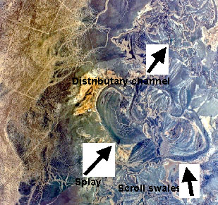


Figure 5.8 Examples of floodplain features, identified from aerial photographs and in the field.
Variable modified from the River Habitat Audit Procedure (Anderson, 1993a).
Bank shape
| VARIABLE NAME | Bank shape |
| CATEGORY | Bank characteristics |
| CONTROL OR RESPONSE | Response |
| OFFICE OR FIELD | Field |
| UNITS OF MEASUREMENT | Choice of five categories |
| INDICATES | The shape of the bank is related to the conveyance of water along the channel. |
Choose one category that represents the predominant shape of the left and right banks along the length of the sampling site.
| concave | |
| convex | |
| stepped | |
| wide lower bench | |
| undercut |
Variable derived from the River Habitat Audit Procedure (Anderson, 1993a).
Bank slope
| VARIABLE NAME | Bank slope |
| CATEGORY | Bank characteristics |
| CONTROL OR RESPONSE | Response |
| OFFICE OR FIELD | Field |
| UNITS OF MEASUREMENT | Choice of five categories |
| INDICATES | The slope of the bank is related to the conveyance of water along the channel, and to the susceptibility of the bank to erosion |
Choose one category that represents the predominant slope of the left and right banks along the length of the sampling site.
| vertical Slope 80-90� | |
| steep Slope 60-80� | |
| moderate Slope 30-60� | |
| low Slope 10-30� | |
| flat Slope <10� |
Variable derived from the River Habitat Audit Procedure (Anderson, 1993a).
Bank material
| VARIABLE NAME | Bank material |
| CATEGORY | Bank characteristics |
| CONTROL OR RESPONSE | Response |
| OFFICE OR FIELD | Field |
| UNITS OF MEASUREMENT | % composition of seven sediment sizes |
| INDICATES | Banks composed of certain sediment types may be more susceptible to erosion |
At each cross section, visually assess the percent composition of the bank sediments within the area lying 5m either side the cross-section. Left and right banks are assessed separately. Where the channel has a distinct upper and lower bank (i.e. benches), assess the lower bank only. The total composition of each of the following seven sediment size categories should equal 100%.
| Sediment category | Size |
| Bedrock | |
| Boulder | > 256mm |
| Cobble | 64 � 256mm |
| Pebble | 16 � 64mm |
| Gravel | 2 � 16mm |
| Sand | 0.06 � 2mm |
| Fines (silt and clay) | < 0.06mm |
Variable derived from the River Habitat Audit Procedure (Anderson, 1993a).
Bedrock outcrops
| VARIABLE NAME | Bedrock outcrops |
| CATEGORY | Bank characteristics |
| CONTROL OR RESPONSE | Response |
| OFFICE OR FIELD | Field |
| UNITS OF MEASUREMENT | % cover of bedrock along banks |
| INDICATES | Presence of bedrock may protect banks from erosion |
At each sampling site, visually assess the percentage of the left and right banks that contain bedrock outcrops (Figure 5.9 and 5.10).

Figure 5.9 Example calculation of the percentage of bedrock outcrops along the banks of a sampling site that is 500m in length. On the left bank, the percent bank cover by bedrock outcrops is 24% (total 120m of bedrock outcrop along 500m of bank) and on the right bank, the percent cover is 30% (total 150m of bedrock outcrop along 500m of bank). The diagram is not to scale.

Figure 5.10 Example of a bedrock outcrop located along a bank. Note that the left bank contains bedrock outcrops but the right bank does not.
Artificial bank protection measures
| VARIABLE NAME | Artificial bank protection measures |
| CATEGORY | Bank characteristics |
| CONTROL OR RESPONSE | Response |
| OFFICE OR FIELD | Field |
| UNITS OF MEASUREMENT | Choice of ten categories |
| INDICATES | Presence of structures that have been built to protect the bank from erosion. |
At each sampling site, indicate the presence of one or more of the following bank protection features:
Variable modified from the River Habitat Audit Procedure (Anderson, 1993a).
Factors affecting bank stability
| VARIABLE NAME | Factors affecting bank stability |
| CATEGORY | Bank characteristics |
| CONTROL OR RESPONSE | Response |
| OFFICE OR FIELD | Field |
| UNITS OF MEASUREMENT | Choice of eleven categories |
| INDICATES | Factors that may contribute to bank erosion and instability |
At each sampling site, indicate the presence of one or more of the following factors that may negatively influence the stability of either the left or right banks:
| Category | Example1 |
| Flow and waves | Bow waves from boats, or waves from turbulent flows |
| Seepage | From a landfill, water storage etc. |
| Runoff | Increased runoff from adjacent land that is unvegetated |
| Stock access | Cattle, sheep or horse access to the channel |
| Human access | Recreation point such as a picnic area or boat ramp |
| Feral animals | Goat, buffalo or horse access to the channel |
| Ford, culvert or bridge | Presence of bridges, culverts or fords that change channel dynamics |
| Clearing of vegetation | Forestry activity, land clearance to create grazing areas, riparian vegetation removal etc. |
| Reservoir release or irrigation offtake regime | Rapid release or draw down of instream flows that may increase the potential for bank slumping |
| Mining | Including gravel or sand extraction, existing or recent mining operations etc. |
| Drain pipes | Stormwater or waste-water pipes that may increase local discharge or turbulence |
| None | Banks are in excellent condition and are not impacted by any of the above factors |
1 Examples are not exhaustive
Variable modified from the River Habitat Audit Procedure (Anderson, 1993a).
Large woody debris
| VARIABLE NAME | Large woody debris |
| CATEGORY | Instream vegetation and organic matter |
| CONTROL OR RESPONSE | Response |
| OFFICE OR FIELD | Field |
| UNITS OF MEASUREMENT | % cover of sampling site |
| INDICATES | Large woody debris is an important ecological component of lowland and upland streams, and can alter flow and other channel characteristics |
Visually estimate the percent cover of large woody debris within the bankfull channel area, along a length of stream that is equal to the length of the sampling site.
Large woody debris is defined as logs and branches that are greater than 10cm in diameter and greater than 1m in length (Gippel, 1995).
Macrophyte cover
| VARIABLE NAME | Macrophyte cover |
| CATEGORY | Instream vegetation and organic matter |
| CONTROL OR RESPONSE | Response |
| OFFICE OR FIELD | Field |
| UNITS OF MEASUREMENT | % cover of different macrophyte types |
| INDICATES | Macrophytes are an important ecological component of streams and can alter flow and other channel characteristics. |
At each sampling site, visually estimate the percentage of the stream area covered by submerged, floating and emergent macrophyte types of any species (Figure 5.11). Stream area is equivalent to the length of the sampling site and the width of the wetted channel (under baseflow conditions).


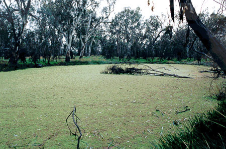
Figure 5.11 Examples of macrophyte types: submerged (top), emergent (middle) and floating (bottom).
Variable derived from the River Habitat Audit Procedure (Anderson, 1993a).
Macrophyte species composition
| VARIABLE NAME | Macrophyte species composition |
| CATEGORY | Instream vegetation and organic matter |
| CONTROL OR RESPONSE | Response |
| OFFICE OR FIELD | Field |
| UNITS OF MEASUREMENT | % cover of different macrophyte species |
| INDICATES | Macrophytes are an important ecological component of streams, and can alter flow and other channel characteristics. |
Record the presence of the common macrophyte species1 at the sampling site and indicate which of these are exotic species. The field guide titled "A Field Guide to Waterplants in Australia" (Sainty and Jacobs, 1994) will assist in macrophyte identification. If any species present at a site is unknown, collect a sample for identification at a later time.
Then, for each of the species present, both native and exotic, visually estimate the percent cover of this species within the stream area. Stream area is equivalent to the length of the sampling site and the width of the wetted channel (under baseflow conditions).
1 The macrophyte taxa initially included on the data sheets are a guide only and may need to be adjusted to suit regional conditions.
Shading of channel
| VARIABLE NAME | Shading of channel |
| CATEGORY | Riparian vegetation |
| CONTROL OR RESPONSE | Response |
| OFFICE OR FIELD | Field |
| UNITS OF MEASUREMENT | Choice of five % shading categories |
| INDICATES | The amount of light reaching the channel is important for instream ecological processes and is an indirect relative measure of riparian vegetation density |
At each sampling site, visually estimate the percentage of the stream area that would be shaded by riparian vegetation when the sun is directly overhead (Figure 5.12). The stream area is equivalent to the length of the sampling site and the width of the wetted channel (under baseflow conditions).
 |
 |
Figure 5.12 Examples of channel shading: <5% shading (left) and >76% shading (right).
Variable derived from AUSRIVAS
Extent of bank trailing vegetation
| VARIABLE NAME | Extent of bank trailing vegetation |
| CATEGORY | Riparian vegetation |
| CONTROL OR RESPONSE | Response |
| OFFICE OR FIELD | Field |
| UNITS OF MEASUREMENT | Choice of four categories |
| INDICATES | Vegetation that trails from the bank into the water provides an important habitat for aquatic biota |
Visually estimate the occurrence and density of trailing bank vegetation along the length of the sampling site as one of the following categories:
| nil | slight | moderate | extensive |
Trailing bank vegetation is the component of the terrestrial riparian vegetation that has direct contact with the water (under baseflow conditions) and which provides habitat and shelter for macroinvertebrates and fish (Figure 5.13). Trailing bank vegetation is generally found along the banks of slow flowing areas such pools and backwaters, although it is often present on the banks of riffles and runs.
 |
 |
Figure 5.13 Examples of trailing bank vegetation: extensive (left) and nil (right).
Variable derived from AUSRIVAS
Riparian zone composition
| VARIABLE NAME | Riparian zone composition |
| CATEGORY | Riparian vegetation |
| CONTROL OR RESPONSE | Response |
| OFFICE OR FIELD | Field |
| UNITS OF MEASUREMENT | % cover of different riparian components |
| INDICATES | Riparian vegetation is important for lateral stability of the channel and has a direct relationship to many aspects of channel character. |
The riparian zone is defined as the area from the water's edge (under baseflow conditions) to a distance from the bank where the stream still interacts with and influences the type and density of the bank-side vegetation (Nichols et al., 2000).
At each sampling site, identify the riparian zone and visually estimate the percentage area of the riparian zone that is covered by each of the following components:
| trees >10m in height |
| trees <10m in height |
| shrubs |
| grasses, ferns and sedges |
The percent cover of each of these four vegetation components within the riparian zone is estimated in planview for the left and right banks together, along the entire length of the sampling site. Schematic drawings to assist in determining the relative percent cover of vegetation are provided in Figure 5.14. Because of the 'layering' effect found within the riparian zone (ie. shrubs can grow under trees, grasses can grow under trees etc.), the sum total percent cover of all four vegetation components may be greater than 100%, but must follow two rules:
Both native and exotic species should be included in the assessment of riparian composition. Where known, include a description of the main species present or the main vegetation types present (e.g. native grasses, rainforest, willows, river red gum, tea tree, casuarina, blackberries, paragrass etc.) in each vegetation component.
Variable derived from AUSRIVAS
Figure 5.14 Schematic diagrams of 1%, 5%, 10%, 20%, 40%, 60% and 80% vegetative cover within the riparian zone. These schematic diagrams are used in conjunction with the riparian zone composition and native and exotic riparian vegetation variables. Drawings are modified from schematic diagrams presented in White and Ladson (1999), and are reproduced with kind permission of the Department of Natural Resources and Environment, Victoria.
1% COVER

5% COVER

10% COVER

20% COVER

40% COVER

60% COVER

80% COVER

Native and exotic riparian vegetation
| VARIABLE NAME | Native and exotic riparian vegetation |
| CATEGORY | Riparian vegetation |
| CONTROL OR RESPONSE | Response |
| OFFICE OR FIELD | Field |
| UNITS OF MEASUREMENT | % cover of native and exotic vegetation |
| INDICATES | The relationship between channel character and riparian vegetation changes with a shift from native to exotic vegetation. |
At each sampling site, visually estimate the percent cover of native and exotic riparian vegetation for the left and right banks together, along the entire length of the sampling site. Schematic drawings to assist in determining the relative percent cover of vegetation are provided in Figure 5.14. Percent native vegetation and percent riparian vegetation must total 100%, regardless of the density of the riparian vegetation at the sampling site.
Variable derived from AUSRIVAS
Regeneration of native woody vegetation
| VARIABLE NAME | Regeneration of native woody vegetation |
| CATEGORY | Riparian vegetation |
| CONTROL OR RESPONSE | Response |
| OFFICE OR FIELD | Field |
| UNITS OF MEASUREMENT | Choice of three categories |
| INDICATES | Regeneration of woody vegetation is related to the recovery of the riparian zone from previous disturbance |
Along the length of each sampling site, visually assess the regeneration of native woody vegetation on the left and right banks together. Do not assess vegetation on instream islands, but include vegetation on bars joined to the banks. Native woody vegetation is defined as immature woody plants under 1m in height.
To measure this variable, first assess whether the sampling site is located in an undisturbed forest1 that has no evidence of clearing, weeds, stock access at any time or other disturbances to the banks such as campgrounds or picnic areas. It is assumed that these sites would have natural rates of regeneration.
If the site is not located in an undisturbed forest, assess the regeneration of native woody vegetation as one of the following categories. Photos are provided in Figure 5.15 to aid in the interpretation of this variable.
| Category | Description |
| Abundant & healthy (>5% cover) | Greater than 5% cover of healthy native regeneration. At least a few taxa of native woody vegetation present, with a range of plant heights and no obvious signs of stress or extensive predation from stock, rabbits, insects etc. |
| Present | Between 1% and 5% cover of native regeneration, or greater than 1% of unhealthy regeneration. Few taxa of woody vegetation present, most regeneration around the same height and obvious signs of stress or extensive predation from stock, rabbits, insects etc. (as evidenced by many eaten or browned leaves) |
| Very limited (<1% cover) | Less than 1% cover of native regeneration |
1 At sites located in areas that would not naturally contain woody vegetation in the riparian zone (eg. frost hollows, native grasslands), substitute woody vegetation with an equivalent type of vegetation. Make a note on the data sheet that this substitution has been made.
Variable derived from the Index of Stream Condition (White and Ladson, 1999 and Department of Natural Resources and Environment, Victoria)
Figure 5.15. Examples of regeneration of indigenous woody vegetation for three categories: a) abundant and healthy, b) present and c) very limited. Dots show the regeneration of native woody vegetation. Examples are taken from Ladson and White (1999) and are reproduced with kind permission of the Department of Natural Resources and Environment, Victoria.
a. Abundant and healthy

Extensive regeneration in healthy condition along the face of the bank. A few species present.

Greater than 5% cover on bar of regeneration in healthy condition.
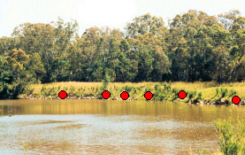
Extensive healthy regeneration along the face of the bank.

Two rows of healthy swamp paperbark planted along a bank.
Figure 5.15. a Examples of regeneration of indigenous woody vegetation for category abundant and healthy (above)
b. Present
 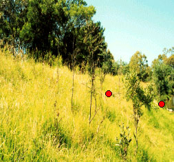 
|  |
| Figure 5.15. b Examples of regeneration of indigenous woody vegetation for category: Present (above) | |
c. Very limited regeneration

This land grazed to the edge of the stream and there is no regeneration of indigenous woody vegetation.

No native regeneration is present under these willows.
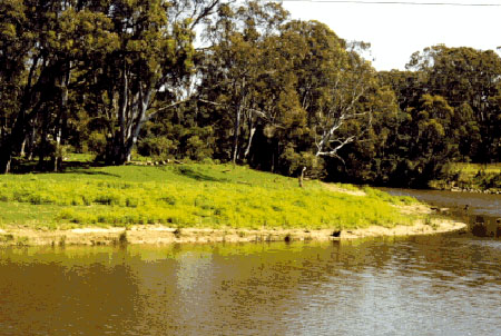
This land is also grazed to the edge of the stream and there is no regeneration.

Infestation of exotic woody vegetation (blackberry gorse). No native regeneration.
Figure 5.15. c Examples of regeneration of indigenous woody vegetation for category: Very limited regeneration (above)
Riparian zone width
| VARIABLE NAME | Riparian zone width |
| CATEGORY | Riparian vegetation |
| CONTROL OR RESPONSE | Response |
| OFFICE OR FIELD | Field |
| UNITS OF MEASUREMENT | m |
| INDICATES | Riparian vegetation is important for lateral stability of the channel and has a direct relationship to many aspects of channel character (Brierley et al., 1996) |
The riparian zone is defined as the area from the water's edge (under baseflow conditions) to a distance from the bank where the stream still interacts with and influences the type and density of the bank-side vegetation (Nichols et al., 2000).
At each cross-section, estimate the width of the riparian zone on the left and right banks separately. It is preferable to measure distances with a tape measure at a number of sites, until estimates can be made with accuracy. The left and right bank measures of riparian zone width should be averaged to give an overall riparian width for the sampling site (Figure 5.16).

Figure 5.16 Example calculation of riparian zone width at a sampling site with three cross-sections. Readings of riparian zone width are made at each cross-section and averaged. In the above example, the average width of the riparian zone on the left bank is 33m and the average width of the riparian zone is 27m on the right bank. Overall average riparian width is 30m.
Variable derived from AUSRIVAS
Longitudinal extent of riparian vegetation
| VARIABLE NAME | Longitudinal extent of riparian vegetation |
| CATEGORY | Riparian vegetation |
| CONTROL OR RESPONSE | Response |
| OFFICE OR FIELD | Field |
| UNITS OF MEASUREMENT | Choice of six categories |
| INDICATES | Patchiness of riparian vegetation, which in turn, indicates previous disturbance or clearance of the riparian zone |
Along the length of each sampling site, visually assess the longitudinal extent, or patchiness, of the riparian zone on the left and right banks separately. Include only the tree and shrub layer components (native or exotic) in the assessment of longitudinal extent, and disregard the ground cover layer. However, for sites where the riparian zone is naturally composed entirely of native grasses, either along the entire site length or in significant patches, include grasses in the assessment of longitudinal extent.
| Assess longitudinal extent of riparian vegetation using one of the following categories | ||
|---|---|---|
| Category | Description and examples1 (shown for one bank only) | |
| None | ||
| No trees or shrubs, only exotic grasses or pasture | ||
| Isolated / scattered | ||
| Isolated trees or shrubs among exotic grasses or pasture | ||
| Regularly spaced, single | ||
| Planted poplars | ||
| Occasional clumps | ||
| Clumps of tea tree scrub among exotic grasses or pasture | ||
| Semi-continuous | ||
| Native forest with cleared areas of exotic grasses | ||
| Continuous | ||
| Undisturbed native forest, river red gum canopy | ||
1 Examples of vegetation types are not exhaustive
Variable derived from the River Habitat Survey (Raven et al., 1998)
Overall vegetation disturbance rating
| VARIABLE NAME | Overall vegetation disturbance rating |
| CATEGORY | Riparian vegetation |
| CONTROL OR RESPONSE | Response |
| OFFICE OR FIELD | Field |
| UNITS OF MEASUREMENT | Choice of six categories |
| INDICATES | Even with an intact riparian zone, vegetation on the land adjacent to the riparian zone can influence characteristics of the stream channel |
This variable considers the condition of the riparian zone and the surrounding valley vegetation simultaneously. The riparian zone is the portion of vegetation that interacts with the stream (see riparian zone composition variable for full definition) and the valley vegetation is the vegetation that is present in the valley in which the channel sits. At each sampling site, assess the condition of the riparian and valley vegetation on the left and right sides together, as one of the following categories:
| Category | Riparian vegetation | Valley vegetation |
 Extreme disturbance | Absent or severely reduced. Vegetation present is extremely disturbed (ie. dominated by exotic species with native species rare or completely absent) | Agriculture and/or cleared land BOTH sides. Plants present are virtually all exotic species (willows, pines, blackberries etc.) |
 Very high disturbance | Some native vegetation present, but it is severely modified BOTH sides by grazing or the intrusion of exotic species. Native species severely reduced in number and cover. | Agriculture and/or cleared land BOTH sides. Plants present are virtually all exotic species (willows, pines, blackberries etc.) |
 High disturbance | Riparian vegetation moderately disturbed by stock or through the intrusion of exotic species, although some native species remain | Agriculture and/or cleared land on ONE side, native vegetation on the other side clearly disturbed or with a high percentage of introduced species present. |
| Note: Sites with valley vegetation cleared BOTH sides but with riparian vegetation in good condition (eg. fenced off from stock) should be included in this category | ||
 Moderate disturbance | Native vegetation on BOTH sides with canopy intact or with native species widespread and common in the riparian zone. The intrusion of exotic species is minor and of moderate impact | Agriculture and/or cleared land on ONE side, native vegetation on the other in reasonably undisturbed state |
 Low disturbance | Native vegetation present on BOTH sides of the river and in relatively good condition with few exotic species present. Any disturbance present is relatively minor. | Native vegetation present on BOTH sides of the river, with a virtually intact canopy and few exotic species. |
 Very low disturbance | Native vegetation on both sides of the river in an undisturbed state. Exotic species are absent or rare. Representative of natural vegetation in excellent condition. | Native vegetation present on both sides of the river with an intact canopy. Exotic species are absent or rare. Representative of natural vegetation in excellent condition. |
Variable derived from the River Habitat Audit Procedure (Anderson, 1993a).
Local impacts on streams
| VARIABLE NAME | Local impacts on streams |
| CATEGORY | Site observations |
| CONTROL OR RESPONSE | Response |
| OFFICE OR FIELD | Field |
| UNITS OF MEASUREMENT | Choice of seventeen categories |
| INDICATES | Local activities that may be impacting on stream habitat |
Indicate whether one or more of the following activities or potential impacts are present at the sampling site or in the local area. Where possible, include a brief description of each selected impact. For example, grazing may be by sheep or cattle, water extraction may be irrigation or rural domestic, litter may be urban rubbish or old car bodies etc.
| sand or gravel mining |
| other mining |
| road |
| bridge / culvert / wharf |
| ford / ramp |
| discharge pipe |
| forestry activities |
| sugar mill |
| sewage effluent |
| irrigation run-off or pipe outlet |
| channel straightening |
| river improvement works |
| water extraction |
| dredging |
| grazing |
| litter |
| recreation |
| other |
Variable derived from the River Habitat Audit Procedure (Anderson, 1993a).
Turbidity (visual assessment)
| VARIABLE NAME | Turbidity (visual assessment) |
| CATEGORY | Site observations |
| CONTROL OR RESPONSE | Response |
| OFFICE OR FIELD | Field |
| UNITS OF MEASUREMENT | Choice of four categories |
| INDICATES | Water clarity and the presence of suspended material in the water |
At each sampling site, visually assess the turbidity of the water as one of the following categories:
| Category | Description |
| clear | water very clear in pools and shallows |
| slight | water slightly turbid in pools and/or shallows |
| turbid | water moderately turbid in pools and/or shallows |
| opaque | water very turbid in both pools and shallows |
Turbidity refers to the relative clarity of water and measures the extent to which light penetration is reduced from suspended materials such as clay, mud, organic matter or plankton. The presence of dissolved materials derived from plant leachates can also reduce water clarity (e.g. blackwater streams) and in such cases, water will be 'tea' coloured. The type of material causing any reduction in water clarity should be noted on the data sheet at each sampling site.
Variable derived from AUSRIVAS
Water level at the time of sampling
| VARIABLE NAME | Water level at the time of sampling |
| CATEGORY | Site observations |
| CONTROL OR RESPONSE | Response |
| OFFICE OR FIELD | Field |
| UNITS OF MEASUREMENT | Choice of five categories |
| INDICATES | Whether flows are elevated or reduced at the time of sampling |
At each sampling site, indicate the water level on the day of sampling as one of the following categories. Water level should be measured relative to the baseflow water mark, which is evidenced by the limit of terrestrial grasses, eroded area or boundary changes in bank sediments.
| Category | Description |
| Dry | Dry channel |
| No flow | Water present but flow is severely or completely reduced |
| Low | Flow at time of sampling lower than baseflow water mark |
| Baseflow | Flow at time of sampling equal or almost equal to baseflow water mark |
| High | Flow at time of sampling substantially higher than baseflow water mark |
| Flood | Flood conditions. Sampling not recommended. |
Variable derived from AUSRIVAS
Sediment oils
| VARIABLE NAME | Sediment oils |
| CATEGORY | Site observations |
| CONTROL OR RESPONSE | Response |
| OFFICE OR FIELD | Field |
| UNITS OF MEASUREMENT | Choice of four categories |
| INDICATES | Chemical pollution |
At each sampling site, examine the sediment and visually assess the presence of oily residues as one of the following categories:
| absent | light | moderate | profuse |
Variable derived from AUSRIVAS
Water oils
| VARIABLE NAME | Water oils |
| CATEGORY | Site observations |
| CONTROL OR RESPONSE | Response |
| OFFICE OR FIELD | Field |
| UNITS OF MEASUREMENT | Choice of five categories |
| INDICATES | Chemical pollution |
At each sampling site, note the presence of oils on the water surface as one of the following categories:
| slick | sheen | globs | flecks | none |
Variable derived from AUSRIVAS
Sediment odours
| VARIABLE NAME | Sediment odours |
| CATEGORY | Site observations |
| CONTROL OR RESPONSE | Response |
| OFFICE OR FIELD | Field |
| UNITS OF MEASUREMENT | Choice of six categories |
| INDICATES | Chemical pollution or deoxygenation in the sediments |
At each sampling site, take a scoop of sediment and smell for odours that correspond to one or more of the following categories:
| normal odour / no odour1 |
| sewage |
| petroleum |
| chemical |
| anaerobic2 |
| other |
1 Unpolluted sediments may have a naturally 'earthy' odour
2 Hydrogen sulphide ('rotten egg gas') is an odour commonly encountered in anaerobic, or deoxygenated, sediments
Variable derived from AUSRIVAS
Water odours
| VARIABLE NAME | Water odours |
| CATEGORY | Site observations |
| CONTROL OR RESPONSE | Response |
| OFFICE OR FIELD | Field |
| UNITS OF MEASUREMENT | Choice of five categories |
| INDICATES | Chemical or organic pollution in the water |
At each sampling site, note the presence of any odours emanating from the water, as one or more of the following categories:
| normal odour / no odour |
| sewage |
| petroleum |
| chemical |
| other |
Variable derived from AUSRIVAS
WATER CHEMISTRY
There are a large number of chemical variables that can be measured to indicate specific aspects of water quality. The physical assessment protocol provides a method for the assessment of physical stream condition and as such, emphasis has been placed on physical, rather than chemical components. However, several basic water quality variables have been included in the protocol, to correspond with those measured in AUSRIVAS. The rationale for inclusion of these variables is both biological and physical. For example, dissolved oxygen, pH, temperature and turbidity can effect the structure and composition of biological communities, whereas conductivity and turbidity are indirect indicators of fluvial processes occurring within a river system. Total phosphorus and total nitrogen broadly describe the nutrient status of the stream and may be direct or indirect indicators of human or agricultural impacts on streams. Other water quality variables can be added to the protocol to suit specific State or Territory conditions.
Each of these water quality variables is measured instantaneously on the day of sampling and can be used to flag impacts that may effect biological communities (e.g. low dissolved oxygen), or to flag impacts that may indicate the physical condition of the surrounding catchment (e.g. high turbidity). In addition, these basic water quality variables can be compared against existing long-term water quality monitoring data, or to guideline levels reported in the Australian and New Zealand Guidelines for Fresh and Marine Water Quality. These guidelines can be accessed via the Environment Australia home page at http://www.environment.gov.au/science/water/
While it is important to measure basic water quality variables when at a sampling site, these instantaneous measurements can not be used as response variables in a predictive model, because they are generally highly variable over diurnal, seasonal and long-term time spans. However, where long-term water quality monitoring data (or modelled water quality data) are available for all reference sites, long-term average values can be used as a response variable. Then, instantaneous measurements of water quality at a test site are valid and can be compared against the average long -term values contained in the reference site database.
Basic water chemistry and nutrients1
| VARIABLE NAME | Basic water chemistry and nutrients1 |
| CATEGORY | Site observations |
| CONTROL OR RESPONSE | Response |
| OFFICE OR FIELD | Field |
| UNITS OF MEASUREMENT | Various |
| INDICATES | Status of pH, conductivity, temperature, dissolved oxygen, conductivity, phosphorus and nitrogen at the time of sampling |
1 Other water quality variables can be included if required by each State or Territory.
The basic water chemistry variables measured at each sampling site are:
| Variable | Units | Description |
| Temperature | oc | Temperature of the water at the time of sampling. |
| Electrical conductivity | µS cm-1 | Measures the total concentration of inorganic ions (salts) in the water. |
| Dissolved oxygen | mg l-1 | Reflects the equilibrium between oxygen consuming processes (e.g. respiration) and oxygen releasing processes (e.g. photosynthesis). Can also be converted to dissolved oxygen % saturation, which essentially adjusts for altitude and temperature effects on oxygen concentration. |
| Turbidity | NTU or FNU | Measures the presence of suspended particulate and colloidal matter such as suspended clay, silt, phytoplankton and detritus. |
| pH | - | Measure of the acidity or alkalinity of the water. |
| Total phosphorus | mg l-1 | Indicator of nutrient status |
| Total nitrogen | mg l-1 | Indicator of nutrient status |
All water chemistry variables are taken from one place in the sampling site and should be collected before disturbing the streambed by wading around the site.
Water chemistry variables such as temperature, conductivity, dissolved oxygen, pH and turbidity should be measured in the field using an appropriate measurement apparatus (e.g. Hydrolab or hand held meters). When taking a reading, be sure to stand downstream from the measurement apparatus (Figure 5.17), and make sure that any instruments used in the field are correctly calibrated.
Water chemistry variables such as total phosphorus and total nitrogen require the collection of a water sample (Figure 5.17). Be sure to follow the standard procedures for collection of water samples, to avoid sample contamination or deterioration.
 |  |
| Figure 5.17 Collection of water quality variables using a Hydrolab (left) and collection of a water sample for laboratory analysis (right). | |
Filamentous algae cover
| VARIABLE NAME | Filamentous algae cover |
| CATEGORY | Site observations |
| CONTROL OR RESPONSE | Response |
| OFFICE OR FIELD | Field |
| UNITS OF MEASUREMENT | Choice of five % cover categories |
| INDICATES | Excess filamentous algae growth may be indicative of nutrient enrichment |
At each cross-section, visually estimate the percent cover of filamentous algae growing on organic or inorganic substrates within an area of stream 5m either side of the cross-section. Choose one of the following categories that correspond to the percent cover of filamentous algae within the assessment area:
| Category | Equivalent percent cover |
| very low | <10% |
| low | 10 � 35% |
| moderate | 35 � 65% |
| high | 65 � 90% |
| very high | >90% |

Variable derived from AUSRIVAS
Periphyton cover
| VARIABLE NAME | Periphyton cover |
| CATEGORY | Site observations |
| CONTROL OR RESPONSE | Response |
| OFFICE OR FIELD | Field |
| UNITS OF MEASUREMENT | Choice of five % cover categories |
| INDICATES | Excess periphyton growth may be indicative of nutrient enrichment |
At each cross-section, visually estimate the percent cover of periphyton growing on organic or inorganic substrates within an area of stream 5m either side of the cross-section. Choose one of the following categories that correspond to the percent cover of periphyton within the assessment area:
| Category | Equivalent percent cover |
| very low | <10% |
| low | 10 � 35% |
| moderate | 35 � 65% |
| high | 65 � 90% |
| very high | >90% |

Variable derived from AUSRIVAS
Moss cover
| VARIABLE NAME | Moss cover |
| CATEGORY | Site observations |
| CONTROL OR RESPONSE | Response |
| OFFICE OR FIELD | Field |
| UNITS OF MEASUREMENT | Choice of five % cover categories |
| INDICATES | In upland sites, presence of moss may indicate the time since the last high flow event that moved bed sediments |
At each cross-section, visually estimate the percent cover of moss growing on substrates within an area of stream 5m either side of the cross-section. Choose one of the following categories that correspond to the percent cover of moss within the assessment area:
| Category | Equivalent percent cover |
| very low | <10% |
| low | 10 � 35% |
| moderate | 35 � 65% |
| high | 65 � 90% |
| very high | >90% |
Variable derived from AUSRIVAS
Detritus cover
| VARIABLE NAME | Detritus cover |
| CATEGORY | Site observations |
| CONTROL OR RESPONSE | Response |
| OFFICE OR FIELD | Field |
| UNITS OF MEASUREMENT | Choice of five % cover categories |
| INDICATES | Detritus is an important food resource for macroinvertebrates. |
At each cross section, visually estimate the percent cover detritus (sticks less than 10cm diameter and 1m long (ie. not large woody debris), twigs and terrestrially derived vegetation within an area 5m either side of the cross-section. Choose one of the following categories that correspond to the percent cover of detritus within the assessment area:
| Category | Equivalent percent cover |
| very low | <10% |
| low | 10 � 35% |
| moderate | 35 � 65% |
| high | 65 � 90% |
| very high | >90% |
Variable derived from AUSRIVAS
Extent of bars
| VARIABLE NAME | Extent of bars |
| CATEGORY | Physical morphology and bedform |
| CONTROL OR RESPONSE | Response |
| OFFICE OR FIELD | Field |
| UNITS OF MEASUREMENT | % extent of bars |
| INDICATES | Increased bar formation may be associated with increasing sedimentation or reduced instream flows |
A bar is a submerged or exposed ridge-like accumulation of sand, gravel or other alluvial material formed in the channel where a decrease in velocity induces deposition (Armantrout, 1998).
At each sampling site, visually estimate the percentage of the streambed area that protrudes to form a bar of any type (Figure 5.20). Also record the dominant sediment particle size of the bars. Streambed area is equivalent to the length of the sampling site and the width of the wetted channel (under baseflow conditions). Bars can be unattached (e.g. islands) or attached to the banks.

Examples of bars in a river channel

Examples of bars in a river channel
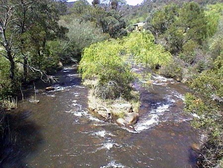
Figure 5.20 Examples of bars in a river channel.
Variable derived from the River Habitat Audit Procedure (Anderson, 1993a).
Type of bars
| VARIABLE NAME | Type of bars |
| CATEGORY | Physical morphology and bedform |
| CONTROL OR RESPONSE | Response |
| OFFICE OR FIELD | Field |
| UNITS OF MEASUREMENT | Choice of nine categories |
| INDICATES | The types of bars present in a channel are indicative of channel behaviour and channel forming processes |
Indicate the presence of one or more of the following bar types along the length of the sampling site:
| bars absent | bars formed around obstructions | ||
| side/point bars VEGETATED | braided channel | ||
| side/point bars UNVEGETATED | infilled channel | ||
 | mid-channel island VEGETATED |  | high flow deposits |
| mid-channel island UNVEGETATED | |||
Variable derived from the River Habitat Audit Procedure (Anderson, 1993a).
Channel shape
| VARIABLE NAME | Channel shape |
| CATEGORY | Physical morphology and bedform |
| CONTROL OR RESPONSE | Response |
| OFFICE OR FIELD | Field |
| UNITS OF MEASUREMENT | Choice of twelve categories |
| INDICATES | The shape of the channel influences many aspects of channel character including discharge, sediment transport and bedform features |
At each sampling site, examine the overall shape of the channel as one of the following categories:
| U shape Most common natural channel type | Box Commonly encountered with severe gully erosion | ||
| Flat U shape | Wide box | ||
| Deepened U shape May be naturally incised channels | V shaped | ||
| Widened or infilled | Trapezoid Engineered channel shape | ||
| Two stage Lowland channel with one bench | Concrete V Engineered channel shape | ||
| Multi stage Lowland channel with >1 bench | Culvert or pipe |
Variable modified from the River Habitat Audit Procedure (Anderson, 1993a).
Bed compaction
| VARIABLE NAME | Bed compaction |
| CATEGORY | Substrate |
| CONTROL OR RESPONSE | Response |
| OFFICE OR FIELD | Field |
| UNITS OF MEASUREMENT | Choice of five categories |
| INDICATES | Partially determines the erodibility or stability of the bed material. |
After examination of the substratum and the bed along the length of the sampling site1, assess the overall character of bed sediment compaction as one of the following categories. The term 'dislodge' refers to the ability to pull individual rocks of different sizes from the streambed with the hands. The term 'overlapping' refers to the relative location of rocks on the streambed (ie. whether they sit on top of each other or next to each other).
| Tightly packed, armoured Array of sediment sizes, overlapping, tightly packed and very hard or impossible to dislodge | |
| Packed, but not armoured Array of sediment sizes, overlapping, tightly packed but can be dislodged with moderate effort | |
| Moderate compaction Array of sediment sizes, little overlapping, some packing but can be dislodged with moderate effort | |
| Low compaction (1) Limited range of sediment sizes, little overlapping, some packing and structure but can be dislodged very easily | |
| Low compaction (2) Loose array of fine sediments, no overlapping, no packing and structure and can be dislodged very easily |
1 In wadeable streams, the bed can be examined visually along the length of the sampling site. In large rivers, the bed should be examined in relation to the range of sediment sizes present at the sampling site (see substrate composition variable). Generally, beds comprised of gravel, sand and silt sediment sizes are not compacted and are easily moved. Thus, these bed types should be allocated to the low compaction (1) or (2) categories.
Variable derived from the River Habitat Audit Procedure (Anderson, 1993a).
Sediment angularity
| VARIABLE NAME | Sediment angularity |
| CATEGORY | Substrate |
| CONTROL OR RESPONSE | Response |
| OFFICE OR FIELD | Field |
| UNITS OF MEASUREMENT | Choice of six categories |
| INDICATES | Indicates the degree of material reworking. |
After visual examination of the substratum and the bed along the length of the sampling site, assess the overall angularity of the cobble, pebble and/or gravel sediment fractions as one of the following categories. Do not include bedrock in the assessment of angularity. Where the cobble, pebble AND gravel fractions are not present at a sampling site (e.g. in lowland rivers), select the 'not present' category.
 | very angular |
 | angular |
 | sub-angular |
 | rounded |
 | well-rounded |
| cobble, pebble and gravel fractions not present |
Variable derived from the River Habitat Audit Procedure (Anderson, 1993a).
Bed stability rating
| VARIABLE NAME | Bed stability rating |
| CATEGORY | Substrate |
| CONTROL OR RESPONSE | Response |
| OFFICE OR FIELD | Field |
| UNITS OF MEASUREMENT | Choice of five categories |
| INDICATES | Whether the bed is eroding or degrading |
The bed stability rating is an assessment of the overall stability of the whole sampling site. The bed stability rating is not a measure of localised patches of deposition or erosion within the sampling site (ie. normal sediment accumulation on a bar located at the inside of a stream bend, White and Ladson, 1999). Rather, this variable asks the question "does the sampling site, as an overall unit, show signs of large scale bed deposition or erosion that may continue outside the bounds of the sampling site?"
With a picture of the links between the sampling site and the surrounding catchment and adjacent river sections in mind, visually assess bed stability at the sampling site as one of the following categories:
| Category | Description | |
 | Severe erosion | Streambed scoured of fine sediments1. Signs of channel deepening. Bare, severely eroded banks. Erosion heads. Steep streambed caused by erosion. |
| Moderate erosion | Little fine sediment1 present. Signs of channel deepening. Eroded banks. Streambed deep and narrow. Steep streambed comprised of unconsolidated (loosely arranged and unpacked) material. | |
| Bed stable | A range of sediment sizes present in the streambed. Channel is in a 'relatively natural' state (not deepened or infilled). Bed and bar sediments are roughly the same size. Banks stable. Streambed comprised of consolidated (tightly arranged and packed) material, may be covered with algae. | |
| Moderate deposition | Moderate build-up of fine sediments1 at obstructions and bars. Streambed flat and uniform. Channel wide and shallow. | |
| Severe deposition | Extensive build up of fine sediments1 to form a flat bed. Channel blocked, but wide and shallow. Bars large and covering most of the bed or banks. Streambed comprised of unconsolidated (loosely arranged and unpacked) material. | |
1 Fine material generally corresponds to the sand, silt and clay sediment fractions

Examples of bed stability. Severe erosion (above)
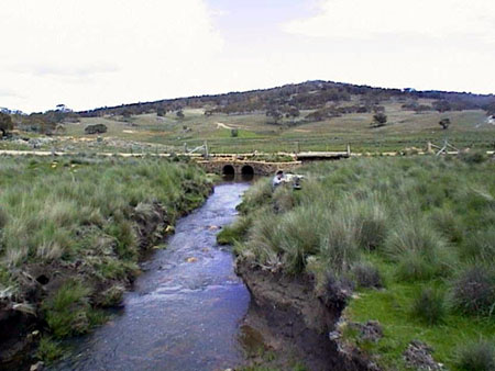
Examples of bed stability. Moderate erosion (above)

Examples of bed stability. Bed stable (above)
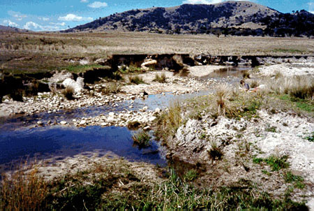
Examples of bed stability. Moderate deposition (above)

Examples of bed stability. Severe deposition (above)
Figure 5.21 Examples of bed stability. Severe erosion, moderate erosion, bed stable, moderate deposition and severe deposition.
Variable modified from the River Habitat Audit Procedure (Anderson, 1993a) and Index of Stream Condition (Ladson and White, 1999 and Department of Natural Resources and Environment, Victoria)
Sediment matrix
| VARIABLE NAME | Sediment matrix |
| CATEGORY | Substrate |
| CONTROL OR RESPONSE | Response |
| OFFICE OR FIELD | Field |
| UNITS OF MEASUREMENT | Choice of five categories |
| INDICATES | The relative composition of the matrix and interstitial components of the streambed sediments |
The sediment matrix variable is derived from sedimentological theories which state that two types of sediment can be characterised on the bed of a river:
Hence, riverbed sediments can be classified into five categories that represent the relationship between the framework and the matrix sediment components: open framework, matrix filled contact framework, framework dilated, matrix dominated and bedrock (Thoms, 1988). These categories also indicate the amount of interstitial space available within the riverbed.
After visual examination of the substratum and the bed along the whole length of the sampling site, assess the overall character of the sediment matrix as one of the following categories:
 | Bedrock |  | Framework dilated 32-60% fine sediment, low availability of interstitial spaces |
 | Open framework 0-5% fine sediment, high availability of interstitial spaces |  | Matrix dominated >60% fine sediment, interstitial spaces virtually absent |
 | Matrix filled contact framework 5-32% fine sediment, moderate availability of interstitial spaces | ||
Substrate composition
| VARIABLE NAME | Substrate composition |
| CATEGORY | Substrate |
| CONTROL OR RESPONSE | Response |
| OFFICE OR FIELD | Field |
| UNITS OF MEASUREMENT | % cover of seven size categories |
| INDICATES | Substrate characteristics are directly related to geomorphological processes and in turn, substrate is a major factor controlling the occurrence of macroinvertebrates. |
Streambed sediment, or substrate, is visually assessed at each sampling site as the percent cover of each of seven size categories, within the area around the cross-section.
The area for assessment of substrate extends for 5m either side of the cross-section transect, regardless of the type of bedform types contained within that area:

Within this 10m long area, assess the relative percent cover of each of the following size classes:
| Sediment category | Size |
| Bedrock | |
| Boulder | > 256mm |
| Cobble | 64 � 256mm |
| Pebble | 16 � 64mm |
| Gravel | 2 � 16mm |
| Sand | 0.06 � 2mm |
| Fines (silt and clay) | < 0.06mm |
The sum of all the substrate categories must equal 100%.
Stream substrate should be assessed to a depth of 10-20cm into the bed. In wadeable streams, sediment should be dislodged and both the surface and sub-surface layers examined. In deep pools or large rivers, sediment should be sampled using a grab sampler or similar device.
Overall substrate composition at the sampling site is calculated separately for each size category by averaging the percent cover obtained at each of the two or three cross-sectional areas used for assessment.

Examples of different sediment classes: cobble (above)

Examples of different sediment classes: gravel and pebble (above)

Examples of different sediment classes: sand and gravel (above).
Figure 5.22 Examples of different sediment classes: cobble (top), gravel and pebble (middle) and sand and gravel (bottom).
Variable derived from AUSRIVAS
What is a cross-section?
In a geomorphological survey, thorough description of the physical characteristics of a stream reach generally includes measurement of several cross-section profiles (Gordon et al., 1992). A channel cross-section is essentially a "slice" through the channel, made at right angles to the flow (Gordon et al., 1992). Data collected at a cross-section provides information on linear and areal channel dimensions. Aspects of channel dimension are related to discharge character and sediment transport, and can also be used to examine changes that occur in the channel profile as a result of anthropogenic or natural events. Aspects of channel dimension can also be used to calculate complex geomorphological or hydrological parameters such as Mannings n or stream power, although these are not included in the current protocol.
What amount of effort and equipment is required to measure a cross-section?
Channel cross-sections can be measured using survey equipment, although in the current protocol, equipment is kept to a minimum (Figure 5.23) and channel cross-sections will be taken using measuring tapes. Regardless of the equipment used, the procedure for measuring cross-sections involves taking vertical measurements at several points across a horizontal transect-line. At each point, both the horizontal distance across the channel and the vertical distance to the streambed are recorded (Figure 5.24). Specific components of the cross-section will be discussed further in the next section.
In wadeable streams, cross-sections are relatively easy to measure because the entire width of the stream can be accessed, even in pools. Accessibility makes cross-sections slightly more difficult to measure in deep pools and large lowland rivers, however, there are many simple ways to sample cross-sections in these types of rivers. For example, in large rivers a boat can be used to access the width of the river or in medium sized rivers, a canoe, small boat or sometimes even a Li-Lo (air mattress) can be used to access the centre of deep pools. When weather, flow and water quality conditions are safe, cross-sections can be performed by swimming across the stream. At some sampling sites, cross-sectional measurements may also be made from a bridge. To take depth measurements along a horizontal transect, a marked pole (e.g. a metre ruler, survey staff or custom made device) can be used, or in slow flowing areas a weighted tape measure or weighted and marked rope is also suitable. Another method that has been used successfully in the River Habitat Audit Procedure (Anderson, 1993a) is to rig a depth sounder onto a rubber flotation board, that can be pushed, pulled or placed across the river to take depth measurements at the required intervals.
It is important that the required numbers of cross-sections are measured at every sampling site. Thus, preparation for a field trip should include planning of the logistics and equipment required to make cross-sectional measurements at all sampling sites, even those located on large or deep rivers. Health and safety issues must be taken into consideration when planning cross-section sampling in any type of river.

Figure 5.23 Equipment required for measuring cross-sections in a wadeable stream. Note that the metre ruler and weighted rope are interchangeable, depending on stream depth. Waders are not shown because wading shoes were used at this site. Additionally, this photo represents the equipment that needs to be carried to assess the whole of a wadeable sampling site, once water quality measurements have been taken.
What does a cross-section look like?
The components that must be measured at each cross-section are detailed in Figure 5.24 and are described as follows:
Stream width at the water surface is the width of the water surface at the time of sampling.
Baseflow stream width is the width of the stream at a point corresponding to baseflow conditions. The baseflow water mark is evidenced by the limit of terrestrial vegetation, eroded area or a break in bank sediment. Under baseflow conditions, baseflow stream width will be equivalent to stream width at the water surface.
Bankfull channel width is the width of the channel between the top of the banks. Bankfull level is the point at the top of the channel where under high flow conditions, the water level would be even with the top of the banks, or in a floodplain river, at the point just before water would spill over onto the floodplain. Further information on the identification of bankfull level is provided in Figure 5.31.
Bank height is the height of the bank measured from the baseflow water mark to the top of the banks. Bank height is measured at both the left and right banks.
Bank width is the width of the bank, extending from the edge of the stream (at the watermark) to the bankfull point. Bank width is measured at both the left and right banks.
Vertical distance between water surface and baseflow water mark is the height difference between the water surface and the baseflow water mark. Vertical distance between water surface and baseflow water mark is measured to compensate for conditions where flow is below normal levels at the time of sampling. This component is measured at both the left and right banks.
Vertical water depths and horizontal distances are measured together at several points across the width of the stream. At each horizontal distance from the edge of the stream, water depth is recorded.
Each of these components are used in various combinations to calculate cross-sectional variables (see section titled 'What variables are derived from a cross-section?') and thus, it is vital to make all of these measurements at each cross-section.
Figure 5.24 Components of a channel cross-section. A tape measure is stretched across the surface of the water and the vertical water depth and horizontal distance from the bank are both measured at several points across the entire channel width. Bank height and the distance between the water surface and the water mark are measured on the left and right sides of the channel. Refer to text for more information.
What is the procedure for measuring a cross-section in the field?
The field procedure for measuring a cross-section is as follows:
In summary, a cross-section requires measurement of the following components:

Figure 5.25 Stretching the tape measure across the stream at the start of a cross-section.

Figure 5.26(a) Measurement of vertical water depths across at a cross-section in a wadeable stream, using a weighted rope or metre ruler.

Figure 5.26(b) Measurement of vertical water depths across at a cross-section in a wadeable stream, using a weighted rope or metre ruler.

Figure 5.27 (a) Measurement of bank height using a metre ruler or metre ruler and tape measure on a wide bank. In the photo on the right, bank width can also be measured with the tape measure.

Figure 5.27 (b) Measurement of bank height using a metre ruler or metre ruler and tape measure on a wide bank. In the photo on the right, bank width can also be measured with the tape measure.

Figure 5.28 (a) Measurement of cross-sections in some difficult wadeable streams. In the top photo the bed was bedrock based and difficult to walk across with the tape measure, so horizontal distances were estimated and depths were measured with a weighted rope. In the bottom photo, the small urban stream was deep and dirty so a survey staff was used to take horizontal distances. Vertical depths were taken using an attached weighted rope.

Figure 5.28 (b) Measurement of cross-sections in some difficult wadeable streams. In the top photo the bed was bedrock based and difficult to walk across with the tape measure, so horizontal distances were estimated and depths were measured with a weighted rope. In the bottom photo, the small urban stream was deep and dirty so a survey staff was used to take horizontal distances. Vertical depths were taken using an attached weighted rope.
How many cross-sections are needed at each sampling site, and where are they placed?
The number and placement of cross-sections at each sampling site is dependent on the relative heterogeneity of the channel.
Homogeneous sampling sites
Two cross-sections should be measured at sampling sites that have a relatively uniform channel shape and sediment composition (Figure 5.29). These types of sampling sites generally correspond to large, low gradient rivers without riffles. The two cross-sections should be placed close to the upstream and downstream boundaries of the sampling site. These cross-sections should not be located on the apex of a bend.
Figure 5.29 Example placement of cross-sections at a homogeneous sampling site. Crosses indicate the apex of bends, where cross-sections should not be placed.
Heterogeneous sampling sites
Three cross-sections should be measured at sampling sites that have a relatively complex channel shape and sediment composition (Figure 5.30). These types of sampling sites generally correspond to small to medium wadeable rivers with a cascade or riffle-pool flow character. The three cross-sections should be placed to represent the different types of bedform units present at the sampling site (ie. riffles, pools, runs) and must include at least one pool. In most streams, appropriate placement of cross-sections would include one riffle, one run and one pool, spread throughout the entire length of the sampling site. Again, cross-sections should not be placed on the apex of a bend.

Figure 5.30 Example placement of cross-sections at a heterogeneous sampling site. Crosses indicate the apex of a bend where cross-sections should not be placed.
How are the bankfull and BASEFLOW water mark levels identified in different channel types?
Accurate identification of the bankfull channel and baseflow water mark levels is fundamental to the measurement of cross-sections. The placement of bankfull and watermark levels at cross-sections located in different channel types is explained in Figure 5.31.
Bankfull channel level is the point within the stream channel where the water level would fill the channel to the tops of the banks. The 'tops of the banks' varies according to channel type (Figure 5.31).
The baseflow water mark level is generally evidenced by the limits of terrestrial vegetation, scour lines, growth of macrophytes or abrupt changes in bank slope (Figure 5.24). However, the baseflow water mark level can be difficult to identify in some situations, using the above criteria. An additional method that can be used to aid the identification of the baseflow water mark level is residual pool depth (Lisle, 1987). Residual pool depth is the difference in depth or bed elevation between a pool and the downstream riffle crest. Residual pool depth is measured by surveying a pool with a tape measure and ruler and subtracting the depth of the riffle crest from those in the pool. A detailed description of the residual pool depth method is available to down load from the United States Forest Service website at http://www.rsl.psw.fs.fed.us/projects/water/Lisle87.pdf
 | Confined upland Confined channels have no floodplain development and are generally found in upland areas with steep valleys. Under undisturbed conditions, bankfull width is usually not much larger than baseflow width. The bankfull level in a confined channel is evidenced by the limit of terrestrial vegetation, the growth of macrophytes, the presence of moss or lichen, the presence of scour marks or an abrupt change in bank slope. (Figure 5pt31 - 1 of 6) |
 | Channelised This type of stream is found where islands (i.e. bars) have formed within the channel. The bars may be vegetated or unvegetated. The placement of a cross-section should run across the bars. Bankfull width should include the bar portion, but baseflow width should break around the bar portion. (Figure 5pt31 - 1 of 6) |
 | Channel with instream bars This type of stream occurs where bars have formed and are attached to the banks. The placement of a cross-section should run across the bars. Bankfull width should include the bar portion, but baseflow width should not include the bar portion if it is not within the baseflow area. (Figure 5pt31 - 1 of 6) |
 | Terraced channel Terraced channels are channels in which the banks are characterised by bench formations. Terraced channels generally occur in lowland floodplain rivers. Regardless of the number of benches present, bankfull width is always measured to the top of the first bench only. (Figure 5pt31 - 1 of 6) |
 | One bank higher than the other When one bank is higher than the other, bankfull width is measured to the top of the lowest bank. This is because the top of the lowest bank represents the point where water would overtop the bank and spill onto the floodplain. (Figure 5pt31 - 1 of 6) |
 | Braided channels Braided channels contain multiple channels that diverge and converge around many islands. Banks may be poorly defined in these types of channels, although the lateral limit of the channel can often be identified. Cross-sectional bankfull width and baseflow width of should be measured across all the threads of a braided channel. (Figure 5pt31 - 1 of 6) |
Figure 5.31. Identification of bankfull level in different channel types. Baseflow water mark level is also drawn on for context, however, the actual position of the water mark level relative to the bankfull level can only be determined after examination in the field.
WHAT VARIABLES ARE DERIVED FROM A CROSS SECTION?
The variables derived from data collected at the cross-sections are given in Table 5.4. Several of these variables are derived directly from field cross-section measurements, several are derived following office-based adjustments and several are derived using the AQUAPAK1 computer package. Instructions for the calculation of each variable are provided in the following pages.
Table 5.4 Variables derived from cross-section data.
| Variable | Derivation |
| Bankfull channel width | Calculated directly from the cross-section data collected in the field |
| Bankfull channel depth | Cross-section data collected in the field is adjusted in the office |
| Baseflow stream width | Taken directly from the cross-section data collected in the field |
| Baseflow stream depth | Cross-section data collected in the field is adjusted in the office |
| Bank width | Calculated directly from the cross-section data collected in the field |
| Bank height | Calculated directly from the cross-section data collected in the field |
| Bankfull width:depth ratio | Calculated using the bankfull channel width and bankfull channel depth variables |
| Bankfull cross-sectional area2 | Calculated in AQUAPAK using adjusted cross-section data |
| Bankfull wetted perimeter2 | Calculated in AQUAPAK using adjusted cross-section data |
| Baseflow cross-sectional area2 | Calculated in AQUAPAK using adjusted cross-section data |
| Baseflow wetted perimeter2 | Calculated in AQUAPAK using adjusted cross-section data |
1 AQUAPAK is a package of stand-alone, IBM compatible computer programs which supplement the text "Stream Hydrology: An Introduction for Ecologists" (Gordon et al., 1992). Among other functions, AQUAPAK calculates the channel cross-sectional area and wetted perimeter variables. AQUAPAK can be purchased for $20 from the Centre for Environmental and Applied Hydrology, Department of Civil and Environmental Engineering, The University of Melbourne, Victoria, 3010. An order form is provided in Appendix 3.
2 Bankfull cross-sectional area and baseflow cross-sectional area are the same variable but calculated for the bankfull and baseflow areas of the channel respectively (Figure 5.24). Likewise, bankfull wetted perimeter and baseflow wetted perimeter are also calculated the same way.
In addition to these variables, substrate composition, bank material, riparian zone width, filamentous algae cover, periphyton cover, moss cover and detritus cover will also be measured in the immediate vicinity of the cross-section. Further information on these variables are provided on each instruction sheet.
Bankfull channel width
| VARIABLE NAME | Bankfull channel width |
| CATEGORY | Cross-sectional dimension |
| CONTROL OR RESPONSE | Response |
| OFFICE OR FIELD | Both |
| UNITS OF MEASUREMENT | m |
| INDICATES | Bankfull stage is an important control on alluvial channels (Gordon et al., 1992) |
Bankfull channel width is recorded directly at each cross-section as the sum of the stream width at the water mark and the left and right bank widths (see Figure 5.24). Bankfull channel width for the sampling site should be calculated as an average of all measurements taken at the two or three cross-sections in each sampling site.
Bankfull channel depth
| VARIABLE NAME | Bankfull channel depth |
| CATEGORY | Cross-sectional dimension |
| CONTROL OR RESPONSE | Response |
| OFFICE OR FIELD | Both |
| UNITS OF MEASUREMENT | m |
| INDICATES | Bankfull stage is an important control on alluvial channels (Gordon et al., 1992) |
Bankfull channel depth is the average depth of the channel at the bankfull level (see Figure 5.24). Calculation of bankfull channel depth at each cross-section involves the addition of bank height to the baseflow stream depth measurements (Figure 5.32).
The overall bankfull channel depth for the sampling site is calculated as the average channel depth of the two to three cross-sections measured at each sampling site.

Figure 5.32 Example calculation of bankfull channel depth for one cross-section. Note that the only the smallest bank height (110cm) is added to the baseflow depths because if the banks are different heights, the smaller value represents the point where the water overtops the banks. Alternatively, the average (left and right) bank height can be added to the baseflow depths. Also, note that baseflow stream depths may have been previously adjusted if the water level at the time of sampling was below baseflow. Refer to the baseflow stream depth variable for information on these adjustments.
Baseflow stream width
| VARIABLE NAME | Baseflow stream width |
| CATEGORY | Cross-sectional dimension |
| CONTROL OR RESPONSE | Response |
| OFFICE OR FIELD | Both |
| UNITS OF MEASUREMENT | m |
| INDICATES | Baseflow stream width is related to the amount of wetted habitat available under baseflow conditions |
Baseflow stream width is recorded directly at each cross-section as the stream width at the water mark (see Figure 5.24). Baseflow stream width for the sampling site should be calculated as an average of all measurements taken at the two or three cross-sections in each sampling site.
Baseflow stream depth
| VARIABLE NAME | Baseflow stream depth |
| CATEGORY | Cross-sectional dimension |
| CONTROL OR RESPONSE | Response |
| OFFICE OR FIELD | Both |
| UNITS OF MEASUREMENT | m |
| INDICATES | Baseflow stream depth is an indicator of channel size, which in turn influences discharge capacity. Baseflow stream depth is also related to the amount of wetted habitat area within the channel. |
Baseflow stream depth is the average depth of the channel at the watermark level (see Figure 5.24). Calculation of baseflow stream depth from the vertical water depth measurements recorded at each cross-section in the field may require some adjustments, to compensate for flows that were below baseflow levels at the time of sampling.
If the water surface at the time of sampling was equal to the baseflow water mark, then baseflow stream depth is simply calculated as the average of all the water depth measurements that were taken across the width of the cross-section.
If the water surface at the time of sampling was below the baseflow water mark, then the water depth measurements must be adjusted up to baseflow levels. To do this, add the vertical distance between the water surface and the baseflow mark to each of the water depth measurements (Figure 5.33).
Regardless of whether adjustments are required at an individual cross section, the overall stream depth for the sampling site is the average depth of the two to three cross-sections measured at each sampling site.

Figure 5.33 Example calculation of adjusted baseflow stream depths, for one cross-section. Note that the left bank vertical distance between the water surface and the baseflow water mark (20cm) is added to the water depths on the left of the channel and the right bank vertical distance (25cm) is added to the water depths on the right of the channel.
Bank width
| VARIABLE NAME | Bank width |
| CATEGORY | Cross-sectional dimension |
| CONTROL OR RESPONSE | Response |
| OFFICE OR FIELD | Both |
| UNITS OF MEASUREMENT | m |
| INDICATES | Represents the width of the bank relative to baseflow stream width. In some situations, overly wide banks may indicate severe erosion. |
Bank width is recorded directly at the left and right banks of each cross-section (see Figure 5.24). Bank width should be averaged for the left and right banks of each cross-section, and then bank width for the sampling site should be calculated as an average of the two or three cross-sections in each sampling site.
Bank height
| VARIABLE NAME | Bank height |
| CATEGORY | Cross-sectional dimension |
| CONTROL OR RESPONSE | Response |
| OFFICE OR FIELD | Both |
| UNITS OF MEASUREMENT | m |
| INDICATES | Bank height is related to channel confinement and to channel volume |
Bank height is recorded directly at the left and right banks of each cross-section (see Figure 5.24). Bank height should be averaged for the left and right banks of each cross-section, and then bank height for the sampling site should be calculated as an average of the two or three cross-sections in each sampling site.
Bankfull width to depth ratio
| VARIABLE NAME | Bankfull width to depth ratio |
| CATEGORY | Cross-sectional dimension |
| CONTROL OR RESPONSE | Response |
| OFFICE OR FIELD | Both |
| UNITS OF MEASUREMENT | Dimensionless |
| INDICATES | Cross sectional channel shape at the bankfull level (Gordon et al., 1992; Armantrout, 1998) which in turn, determines the maximum cross sectional flow that can be transported through the system (Brierley et al., 1996) |
Width to depth ratio (W:D) is calculated for each cross section taken at each sampling site by dividing bankfull channel width by bankfull channel depth (see the bankfull channel width instruction sheet and the bankfull channel depth instruction sheet):
W:D = (W/D)
where:
W = bankfull channel width (m)
D = bankfull channel depth (m)
A width to depth ratio should be calculated for the two or three cross sections taken at a sampling site, and averaged to provide an overall width to depth ratio for the sampling site.
Bankfull cross-sectional area
| VARIABLE NAME | Bankfull cross-sectional area |
| CATEGORY | Cross-sectional dimension |
| CONTROL OR RESPONSE | Response |
| OFFICE OR FIELD | Both |
| UNITS OF MEASUREMENT | m2 |
| INDICATES | Bankfull stage is an important control on alluvial channels (Gordon et al., 1992) |
Bankfull cross-sectional area is calculated for each cross-section using the AQUAPAK computer package. Data are prepared by deriving a set of coordinates from the horizontal distances across the bankfull width of the cross-section and the bankfull stream depth measurements (Figure 5.34). These coordinates are entered into AQUAPAK and bankfull cross-sectional area is calculated using the XSECT program.
The overall bankfull cross-sectional area for the sampling site is calculated as the average area of the two to three cross-sections measured at each sampling site.

These measurements are entered into AQUAPAK as the following coordinates
| Horizontal distance (m) | Bankfull depth (m) |
| 0 | 0 |
| 2.2 | 1.62 |
| 2.7 | 1.67 |
| 3.3 | 1.75 |
| 3.9 | 1.85 |
| 4.5 | 1.85 |
| 5.2 | 1.68 |
| 5.6 | 1.65 |
| 7.8 | 0 |
Figure 5.34 Example derivation of AQUAPAK data for the calculation of bankfull cross-sectional area. Coordinates are comprised of adjusted bankfull horizontal distances and bankfull channel depth measurements. To derive adjusted bankfull horizontal distances, a factor that is equivalent to the width of each bank is added to each of the original baseflow horizontal distances. Instructions on the calculation of bankfull channel depths are provided with the bankfull channel depth variable.
Bankfull wetted perimeter
| VARIABLE NAME | Bankfull wetted perimeter |
| CATEGORY | Cross-sectional dimension |
| CONTROL OR RESPONSE | Response |
| OFFICE OR FIELD | Both |
| UNITS OF MEASUREMENT | m |
| INDICATES | Bankfull wetted perimeter is related to the amount of wetted habitat area within the channel |
Bankfull wetted perimeter is the distance along the streambed and banks under bankfull conditions (Gordon et al., 1992). Wetted perimeter is calculated in the XSECT program of AQUAPAK, using the same coordinates used to calculate bankfull cross-sectional area (see bankfull cross-sectional area variable for instructions on the derivation of coordinates).
Baseflow cross-sectional area
| VARIABLE NAME | Baseflow cross-sectional area |
| CATEGORY | Cross-sectional dimension |
| CONTROL OR RESPONSE | Response |
| OFFICE OR FIELD | Both |
| UNITS OF MEASUREMENT | m2 |
| INDICATES | Baseflow cross-sectional area is an indicator of channel size, which in turn influences discharge capacity. Baseflow cross-sectional area is also related to the amount of wetted habitat area within the channel. |
Baseflow cross-sectional area is calculated for each cross-section using the AQUAPAK computer package. Data are prepared by deriving a set of coordinates from the horizontal distances across the baseflow width of the cross-section and the baseflow stream depth measurements (Figure 5.35). These coordinates are entered into AQUAPAK and baseflow cross-sectional area is calculated using the XSECT program.
The overall baseflow cross-sectional area for the sampling site is calculated as the average area of the two to three cross-sections measured at each sampling site.

These measurements are entered into AQUAPAK as the following coordinates
Horizontal distance (m) | Baseflow depth (m) |
| 0 | 0 |
| 0.4 | 0.52 |
| 0.9 | 0.57 |
| 1.5 | 0.65 |
| 2.1 | 0.75 |
| 2.7 | 0.75 |
| 3.4 | 0.58 |
| 3.8 | 0.55 |
| 4.2 | 0 |
Figure 5.35 Example derivation of AQUAPAK data for the calculation of baseflow cross-sectional area. Coordinates are comprised of the horizontal distances across the baseflow width of the stream and the baseflow depths. Instructions on the calculation of baseflow depths are provided with the baseflow stream depth variable. Note that when there is a difference between baseflow level and water level at the time of sampling, one additional coordinate can be added to each side of the cross-section. On the right side, the vertical coordinate would be the vertical distance between the water surface and the water mark and the horizontal coordinate would be the stream width at the water surface (see Figure 5.24). On the left side, the vertical coordinate would be the vertical distance between the water surface and the water mark and the horizontal coordinate would be the difference between baseflow stream width and stream width at the time of sampling, minus the distance of the first horizontal coordinate measured.
Baseflow wetted perimeter
| VARIABLE NAME | Baseflow wetted perimeter |
| CATEGORY | Cross-sectional dimension |
| CONTROL OR RESPONSE | Response |
| OFFICE OR FIELD | Both |
| UNITS OF MEASUREMENT | m |
| INDICATES | Baseflow wetted perimeter is related to the amount of wetted habitat area within the channel |
Baseflow wetted perimeter is the distance along the streambed under baseflow conditions. Wetted perimeter is calculated in the XSECT program of AQUAPAK, using the same coordinates used to calculate baseflow cross-sectional area (see baseflow cross-sectional area variable for instructions on the derivation of coordinates).
When implemented on a National scale, the AUSRIVAS physical assessment protocol will provide a standardised tool for the assessment of physical stream condition. As such, it is important that the data collected by each State or Territory conforms to the standard methods set out in this protocol. It is desirable to avoid deviations from these methods, because each deviation has the potential to effect the production of robust and reliable predictive models.
As mentioned in Part 3, the collection of field data for the physical assessment protocol is analogous to the collection of macroinvertebrates for the AUSRIVAS models and thus, it is vital that a full set of reliable, high quality data are collected. This protocol contains detailed information about the collection of each office and field based variable (Part 5). This information should be adopted as standard procedure. However, there is a 'conceptual limit' to the types of information that can be portrayed in text and it is essential to extend the content of this manual to a field based learning and training exercise. Training of sampling teams will ensure that the field data is of high quality, is measured in the appropriate format, and is consistent across sampling teams. In turn, these factors will contribute to the reliability and robustness of predictive models.
Field sampling teams, or representative members of each team, should be trained in standard procedure prior to the commencement of reference site sampling. This training exercise will ensure that data collection methods are identical and consistent across sampling teams. Training should be conducted in a range of river types, and should include at least one large river. It is recommended that sampling teams simultaneously attend this training exercise, and confer with each other to standardise a procedure for the collection of each individual variable. Specific aspects of data collection that should be demonstrated and synchronised during the training exercise include:
In addition, some States or Territories may need to add new variables, or make minor modifications to some variables to reflect locally encountered conditions (e.g. macrophyte species). Any additions or modifications must be made cautiously, and updated on the data sheets. All new or modified variables should be included in the training exercise.
Cross-sections in wadeable rivers
Cross-sections in large rivers or deep pools
General
Health and safety equipment1
1 Note that this list is not exhaustive, and should be used as a guide only
AQUAPAK software is a package of stand alone computer programs, written in FORTRAN77, which supplements the text Stream Hydrology: An Introduction for Ecologists by N.D. Gordon, T.A. McMahon and B.L. Finlayson (John Wiley & Sons Ltd., UK, 1992, 526 pp).
The software package includes routines for computing:
The programs are interactive and user-friendly, and can run on IBM compatible personal computers. Many of the programs include graphical output.
To obtain a copy of the software, complete the details below and return to:
AQUAPAK Software
Centre for Environmental Applied Hydrology
Department of Civil & Environmental Engineering
The University of Melbourne
Victoria 3010
AUSTRALIA
or fax to: +61 3 8344 6215
The price of the software is Aus$20.00 or US$15.00 (which includes the cost of two high density 3.5" discs, postage and handling). This may be paid by Bankcard, Mastercard or Visa.
Payment details:
Bankcard / Mastercard / VisaNo: ....................�����..����..........
Name on card: ......................................... Expiry date: ..............................
AQUAPAK to be sent to:
Name: ..............................................................................���..
Organization: ..............................................................................���..
Address: ............................................................................���....
..............................................................................���..
...............�......................���........................................
 Riversinfo Australia (au.riversinfo.org): Publication Information:
Current at December 2002
![]() au.riversinfo.org has been developed to facilitate public access to scientific and technical information on Australia's Rivers. Much of this material was paid for using public funds and is therefore owned by the Australian people. Environment Australia have been instrumental in making available all the publications from:
au.riversinfo.org has been developed to facilitate public access to scientific and technical information on Australia's Rivers. Much of this material was paid for using public funds and is therefore owned by the Australian people. Environment Australia have been instrumental in making available all the publications from:
 The au.riversinfo.org Internet site is in-part supported by the Natural Heritage Trust. The Natural Heritage Trust focuses on five key environmental themes - land, vegetation, rivers, coasts and marine, and biodiversity. The programs of the Natural Heritage Trust play a major role in developing sustainable agriculture and natural resource management, as well as protecting our unique biodiversity through improved management and delivery of resources.
 The au.riversinfo.org Internet site is in-part supported by Sydney Airport who have co-funded a Natural Heritage Trust supported project intended to develop Internet based environmental information integration and management systems. This will assist in developing an overall perspective on the demands and uses for environmental resources


